Polynomial methods / Learn by experiment
Smoothness still controls convergence
Repeat the four regularity experiments on a nonperiodic Chebyshev grid and see when a polynomial becomes exact.
Download runnable lesson (.zip)
Includes the model, inputs, required headers and a short run guide.
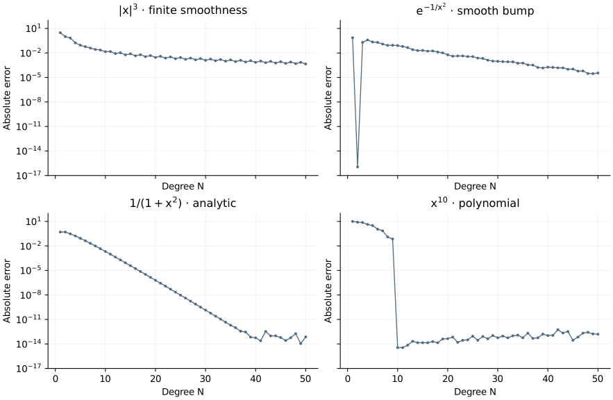
The Fourier smoothness experiment showed four convergence patterns. Program 12 of Trefethen (2000) asks the same question on a finite interval, using polynomials instead of periodic trigonometric interpolants. We repeat all four functions and every degree from 1 to 50.
Four functions with four different promises
| Function | Exact derivative | What to investigate |
|---|---|---|
| \(|x|^3\) | \(3x|x|\) | Limited smoothness produces algebraic convergence. |
| \(e^{-1/x^2}\), defined as zero at \(x=0\) | \(2e^{-1/x^2}/x^3\), also zero at 0 | Infinitely smooth does not mean analytic. |
| \(1/(1+x^2)\) | \(-2x/(1+x^2)^2\) | Complex singularities at \(x=\pm i\) limit geometric convergence. |
| \(x^{10}\) | \(10x^9\) | Degree 10 can represent the function exactly in exact arithmetic. |
At each degree we differentiate the unique polynomial through the samples, then measure the largest error at the nodes:
\[E_N=\max_{0\le j\le N}|(Df)_j-f'(x_j)|. \tag{1}\]
for (int n = 1; n <= maximum; ++n) {
  const auto x = polynomial::nodes(n);
  const auto d = polynomial::differentiation(x);
  for (int type = 0; type < 4; ++type) {
    polynomial::Vector values;
    for (double point : x)
      values.push_back(polynomial::profile(type, point).value);
    const auto derivative = polynomial::apply(d, values);
    double error = 0;
    for (int j = 0; j <= n; ++j)
      error =
          std::max(error, std::abs(derivative[j] -
                                   polynomial::profile(type, x[j]).derivative));
    output << n << ',' << type << ',' << error << '\n';
  }
}
This chapter uses the example-local Chebyshev matrix derived in the differentiation lesson. Its matrix and profile formulas are mathematical reference code; the native OpenPFC FFT comparison is developed there. No public Chebyshev-gradient API is assumed.
Look for the mechanism
openpfc run model.cpp input.json --source-root .. --launcher=noneSet n to the maximum degree. results/regularity.csv has one record per degree and profile; profile numbers follow the table from 0 to 3. The bump and its derivative are assigned their limiting value at zero, avoiding an undefined floating-point expression. Tiny underflowed tails are also zero.
Inspect consecutive odd and even degrees. The two node sets sample the centre differently, so the curves need not decrease monotonically. For the bump, degree 2 has an especially misleading success: its interpolant is \(x^2/e\), whose derivative happens to match the bump at all three nodes. The bump is not a quadratic between those nodes. This explains the isolated low-degree dip without claiming that three samples resolve the function. For \(x^{10}\), verify the sharp improvement at degree 10. An increasing tail at large degree can reflect cancellation and differentiation’s amplification of rounding errors, rather than a loss of smoothness.
The regression checks compare selected matrix actions with an independently constructed Lagrange polynomial derivative and test degree-10 exactness. The plotted error is measured at nodes; it does not directly certify a continuous maximum over the entire interval. Next, turn differentiation around and calculate an integral. The log plot places zero errors at its \(10^{-17}\) display floor; the CSV retains the computed values.
The complete C++ model and starting input are available with this lesson. It also uses the shared collocation.hpp; keep its relative location when saving the files.