Polynomial methods / Learn by experiment
Differentiate a cosine-mapped grid
Compare a Chebyshev collocation matrix with coefficients obtained through OpenPFC LocalFFT, including both endpoints.
Download runnable lesson (.zip)
Includes the model, inputs, required headers and a short run guide.
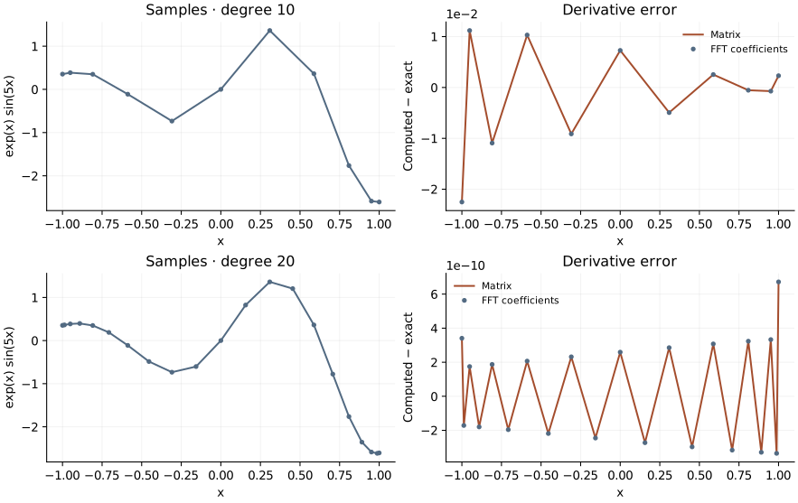
A nonperiodic interval can still benefit from a Fourier transform. Write \(x=\cos\theta\) and observe that a degree-\(N\) polynomial in \(x\) becomes a cosine series in \(\theta\). Programs 11 and 18 of Trefethen (2000) differentiate \(f(x)=e^x\sin(5x)\) on this grid. We compare the collocation matrix with a cosine-coefficient route using OpenPFC’s public LocalFFT.
A derivative matrix from interpolation
Let \(x_j=\cos(j\pi/N)\) and let \(c_0=c_N=2\), with \(c_j=1\) otherwise. For distinct rows and columns,
\[ \begin{gathered} D_{ij}=\frac{c_i}{c_j}\frac{(-1)^{i+j}}{x_i-x_j}, \\ D_{ii}=-\sum_{j\ne i}D_{ij}. \end{gathered} \tag{1}\]
The diagonal enforces the derivative of a constant. Each row acts on every sample; this is global polynomial collocation, not a local stencil.
inline Matrix differentiation(std::span<const double> x) {
  const int n = static_cast<int>(x.size()) - 1;
  Matrix d(n + 1, Vector(n + 1));
  for (int i = 0; i <= n; ++i)
    for (int j = 0; j <= n; ++j) {
      if (i == j) continue;
      const double ci = (i == 0 || i == n) ? 2 : 1;
      const double cj = (j == 0 || j == n) ? 2 : 1;
      d[i][j] = (ci / cj) * ((i + j) % 2 ? -1 : 1) / (x[i] - x[j]);
      d[i][i] -= d[i][j];
    }
  return d;
}
Make an even extension
The sequence \(f(x_0),\ldots,f(x_N),f(x_{N-1}),\ldots,f(x_1)\) has length \(2N\). Its unscaled real FFT yields cosine coefficients: divide interior coefficients by \(N\), and the constant and highest coefficients by \(2N\). If \(p(x)=\sum_k a_kT_k(x)\), then
\[p'(\cos\theta)=\sum_{k=1}^N k a_k\frac{\sin(k\theta)}{\sin\theta}. \tag{2}\]
At \(x=1\), \(T_k'(1)=k^2\); at \(x=-1\), \(T_k'(-1)=(-1)^{k-1}k^2\). These analytic limits avoid dividing by zero at the endpoints.
inline Vector fft_derivative(const Vector &values) {
  const int n = static_cast<int>(values.size()) - 1;
  pfc::fft::LocalFFT fft({2 * n, 1, 1});
  Vector even(2 * n);
  for (int j = 0; j < 2 * n; ++j) even[j] = values[j <= n ? j : 2 * n - j];
  pfc::fft::ComplexVector coefficients(n + 1);
  fft.forward(even, coefficients);
  Vector a(n + 1), derivative(n + 1);
  for (int k = 0; k <= n; ++k)
    a[k] = coefficients[k].real() / ((k == 0 || k == n) ? 2 * n : n);
  // f(cos(theta)) = sum a_k cos(k theta). Differentiate that polynomial.
  for (int j = 0; j <= n; ++j) {
    const double theta = std::numbers::pi * j / n;
    for (int k = 1; k <= n; ++k) {
      const double basis = j == 0 ? k
                                  : (j == n ? (k % 2 ? k : -k)
                                            : std::sin(k * theta) / std::sin(theta));
      derivative[j] += k * a[k] * basis;
    }
  }
  return derivative;
}
OpenPFC supplies the local transform and its normalization contract. The mapping, cosine coefficients, and endpoint formulas are example-owned. Unlike the book’s FFT differentiation routine, this transparent version evaluates the coefficient sum directly at every node, so its total work is \(O(N^2)\) despite using an FFT for coefficient extraction. It demonstrates the same polynomial derivative, without claiming an \(O(N\log N)\) evaluator.
Check an answer, not only agreement
for (int n : sizes) {
  polynomial::degree({{"n", n}});
  const auto x = polynomial::nodes(n);
  polynomial::Vector values;
  for (double point : x) values.push_back(std::exp(point) * std::sin(5 * point));
  const auto dense = polynomial::apply(polynomial::differentiation(x), values);
  const auto transformed = polynomial::fft_derivative(values);
  for (int j = 0; j <= n; ++j) {
    const double exact =
        std::exp(x[j]) * (std::sin(5 * x[j]) + 5 * std::cos(5 * x[j]));
    output << n << ',' << x[j] << ',' << values[j] << ',' << dense[j] << ','
           << transformed[j] << ',' << exact << '\n';
  }
}
openpfc run model.cpp input.json --source-root .. --launcher=noneinput.json selects sizes, initially [10,20]. results/derivatives.csv includes the actual samples, both derivatives and \(e^x(\sin5x+5\cos5x)\). Compare endpoint errors separately from interior errors. The tests check every value against this independent derivative, then require the degree-20 error to be much smaller than degree 10. They also check agreement between the two algorithms; agreement alone would not establish accuracy.
The complete C++ model and starting input are available with this lesson. It also uses the shared collocation.hpp; keep its relative location when saving the files.