Differentiation / Regularity

What smoothness buys you

A method called spectral does not give every function the same convergence curve.

Includes the model, inputs, required headers and a short run guide.

The first differentiation lesson used the analytic function \(e^{\sin x}\). Its rapidly decreasing error is compelling, but it is only one regularity class. Program 7 of Trefethen (2000) asks the more revealing question: what changes when the function changes?

Four functions with known derivatives

On \([0,2\pi)\) compare:

Table 1: The bump and its derivative have limiting value zero at the periodic join; the implementation uses those limits explicitly.

Function	Exact first derivative	Distinguishing property
\(\|\sin x\|^3\)	\(3\sin x\cos x\,\|\sin x\|\)	Only finite smoothness at zeros
\(\exp[-1/\sin^2(x/2)]\)	\(u\sin x/[2\sin^4(x/2)]\)	Smooth, but not analytic at the periodic join
\(1/[1+\sin^2(x/2)]\)	\(-\sin(x/2)\cos(x/2)u^2\)	Analytic in a strip around the real axis
\(\sin(10x)\)	\(10\cos(10x)\)	A single band-limited mode

We measure the maximum derivative error on the grid, using both the cotangent matrix and OpenPFC’s Fourier evaluator. Neither numerical derivative supplies the analytic reference in Table 1.

Why the curves differ

Fourier differentiation multiplies each coefficient by its wavenumber. The error therefore depends on how quickly the coefficients decay. Finite smoothness gives algebraic decay. A smooth nonanalytic bump can converge faster than every fixed algebraic order without having one fixed exponential rate. Analyticity in a complex strip gives exponential decay until roundoff dominates (Trefethen 2000, program 7).

For the last function there is no unresolved tail once the grid can represent mode ten without aliasing. The requirement is \(N>20\). At \(N=20\) the samples of \(\sin(10x)\) vanish, while its derivative does not. That is a useful counterexample to treating a finite grid as the function.

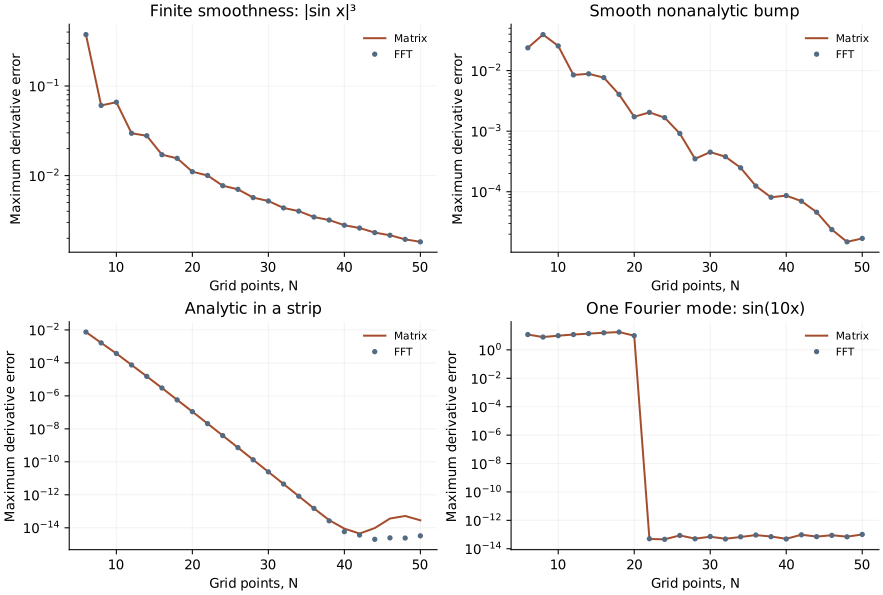
Figure 1: Maximum derivative error versus grid size for the four profiles, computed by the C++ examples. Matrix and FFT evaluate the same interpolating derivative. The single-mode case becomes accurate only beyond its resolution threshold.

Make the comparison explicit

for (int n : sizes) {
  const double h = 2 * std::numbers::pi / n;
  const auto domain = pfc::domain::create(pfc::GridSize{{n, 4, 4}},
                                          pfc::PhysicalOrigin{{0, 0, 0}},
                                          pfc::GridSpacing{{h, 1, 1}});
  pfc::sim::stacks::SpectralCPUStack stack(domain, comm.rank(), comm.size());
  auto &u = stack.u();
  auto derivative = pfc::field::create<Derivative>(u, stack.fft());
  for (const auto &name : names) {
    std::vector<double> samples(n);
    for (int j = 0; j < n; ++j)
      samples[j] = profiles::evaluate(name, j * h).value;
    u.apply([&](double x, double, double) {
      return profiles::evaluate(name, x).value;
    });
    derivative.prepare();
    std::array<double, 3> local{};
    u.for_each_owned([&](int i, int j, int k) {
      const int row = i + u.box().low[0];
      const double exact = profiles::evaluate(name, row * h).derivative;
      const double matrix = profiles::matrix_derivative(samples, row);
      const double fourier = derivative(i, j, k).x;
      local[0] = std::max(local[0], std::abs(matrix - exact));
      local[1] = std::max(local[1], std::abs(fourier - exact));
      local[2] = std::max(local[2], std::abs(matrix - fourier));
    });
    std::array<double, 3> error{};
    MPI_Allreduce(local.data(), error.data(), 3, MPI_DOUBLE, MPI_MAX, comm);
    worst_agreement = std::max(worst_agreement, error[2]);
    if (comm.rank() == 0) {
      output << n << ',' << name << ',' << error[0] << ',' << error[1] << ','
             << error[2] << '\n';
    }
  }
}

The field geometry and derivative request stay fixed within each resolution. Only the profile changes. The global maximum reduction ensures the error includes subdomain edges and every rank’s values.

Reproduce two book experiments

For program 7, use the supplied resolutions 6, 8, …, 50:

openpfc run model.cpp input.json --source-root .. --launcher=none

For program 2’s matrix convergence experiment on \(e^{\sin x}\), use:

openpfc run model.cpp trefethen-p2.json --source-root .. --launcher=none

That input selects the analytic profile at every even resolution from two through 100. We add the FFT comparison to the book’s matrix experiment; we do not substitute one for the other. Both commands write results/smoothness.csv in distinct preserved attempt directories.

First predict the errors at \(N=20\) and \(N=22\) for the band-limited case. Then increase the analytic profile’s resolution beyond the roundoff plateau. Explain why fitting a convergence order there would be misleading. Finally, use two MPI ranks and compare the maximum errors, allowing for small floating-point differences.

Independent verification

The checks reconstruct the derivative using a direct complex DFT in standard-library Python. That calculation uses neither OpenPFC nor the cotangent matrix. It compares the reported matrix and FFT errors at \(N=6,20,22,50\) against independently differentiated sampled profiles. Invalid profile names must fail before entering the evaluator.

The experiment concerns grid-point errors for these functions. It is not a proof of a convergence rate for every smooth function, an arbitrary complex strip, or floating-point arithmetic at unlimited resolution.

The complete C++ model and starting input are available with this lesson. It also uses the shared profiles.hpp; keep its relative location when saving the files. The program 2 resolution preset is also available.

References

Trefethen, Lloyd N. 2000. Spectral Methods in MATLAB. Society for Industrial; Applied Mathematics. https://doi.org/10.1137/1.9780898719598.