Spectral · 3D · div u = 0
Incompressible flow
Periodic Navier-Stokes on the Fourier velocity.
Taylor-Green, decaying turbulence, and constant-power low-mode forcing. The rotational step has a device path.
OpenPFC
OpenPFC is a structured-grid framework for computational physics. Compose a PDE from shared numerical components, then run it from one rank toward GPUs and a cluster.
Phase-field crystal models began the project. Flow, phase fields, elasticity, films, and kinetics now use the same path.
01 — Applications
What you can build on the same grid. The plates are browser drawings. Hover a tile for one extra fact.
Spectral · 3D · div u = 0
Periodic Navier-Stokes on the Fourier velocity.
Taylor-Green, decaying turbulence, and constant-power low-mode forcing. The rotational step has a device path.
Spectral · 3D · density
Tungsten is the main application.
JSON or TOML in. CPU, CUDA, and HIP binaries when the build enables them.
Spectral ETD · conserved
Spinodal dynamics for an Fe-Cr-like solution.
A recorded concentration field from this application is in the next section.
Finite difference · 2D
A small non-conserved phase field.
Optional PNG frames. CUDA or HIP when you compile them.
FD or spectral · 3D
Even difference orders from 2 to 20, or one spectral step.
The same heat equation, two discretizations, one application.
Spectral · Helmholtz-Navier
Size-dependent elasticity on a periodic cell.
Inverse design of a target stiffness is a separate application, shown below as solver output.
Phase field · alloy
Quantitative solidification with solute and microelasticity.
Kobayashi growth with temperature is its own application.
Spectral ETD · surface
Lubrication dewetting on a periodic film.
Mullins surface diffusion and a sixth-order electrohydrodynamic gap are separate applications.
1D2V · kinetics
Electromagnetic kinetics on a reduced phase space.
Landau damping, two-stream, and Weibel.
Spectral · first order
A coupled acoustic wave, displacement plus velocity.
Kawahara is the dispersive sibling. It does not smooth.
Also in the tree: higher-order phase-field crystal and aluminumNew, the FCC phase-field crystal application. The 2D vorticity prototype stays in examples, not in the flow application.
02 — Solver output
Recorded runs, not sketches. The Taylor-Green film is the 512 cubed trajectory. Flat fields use a presentation color scale.
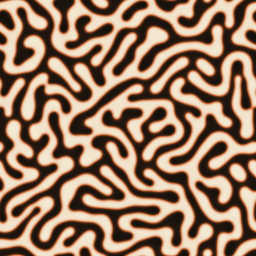
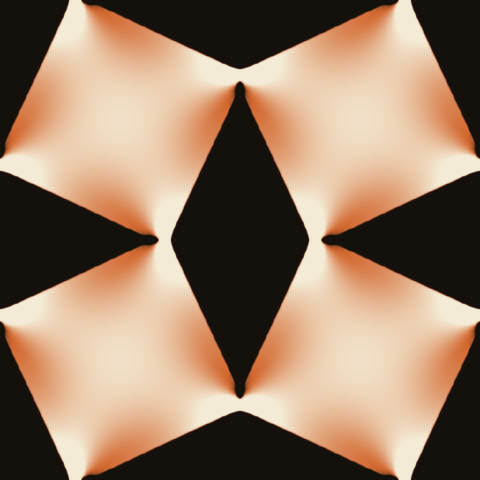
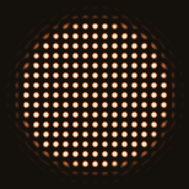
Provenance, commands, and the render script are in the figure provenance. The atlas above is still a drawing.
03 — Scale
Measured heat runs on LUMI-G. One MI250X GCD is one rank, and a node is eight GCDs. Finite difference and distributed FFT do not share one efficiency.
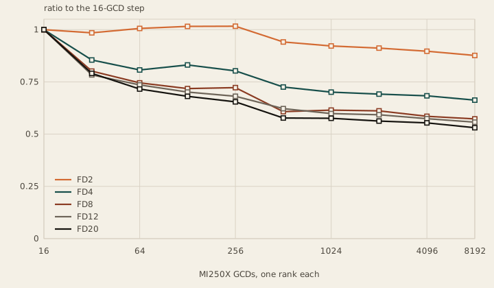
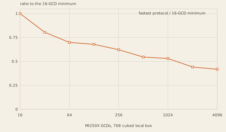
Local finite-difference work scales strongly, and the stencil changes the result. At 8,192 GCDs the 16-GCD baseline reads FD4 66.3%, FD8 57.3%, FD12 55.7%, FD20 53.1%. The same walls against each order's one-node step are 68.4%, 59.0%, 57.5%, and 54.2%. A distributed FFT pays a different communication cost, so it is not a second copy of the FD2 curve. The fastest protocol is not the same one at every width, and that ranking did not change a production selector. These are recorded LUMI-G campaigns, not a re-run of today's master.
04 — Path
The path a problem takes. CUDA and HIP are part of that path, not a later wrapper around the CPU code.
Equations, materials, forcing
FFT, finite difference, Chebyshev, projections, time
Fields, domains, decomposition, halos
CPU, CUDA, HIP
MPI, distributed FFT, the job you launch
One contract, three builds
MPI is on for every supported build. Distributed FFTs go through HeFFTe. Turning HeFFTe off skips the spectral applications and leaves the finite-difference work.
In the repository the dependency runs the other way: runtime depends on the kernel, and the kernel includes no backend. The architecture note is the precise picture, including which owner holds mechanics, constitutive laws, and the incompressible step.
05 — Numerics
Start with a derivative, follow it into a heat equation, then change the numerical choices yourself. Explore the equations and interactive experiments before opening the detailed reference.
Follow Fourier modes through nonlinear products, ETD2 and a verified C++ model. Compare actual serial and MPI results.
Start with samples, compare finite differences with Fourier derivatives, and measure spatial and temporal errors before running C++.
Chebyshev operators, and Poisson and Helmholtz solves.
Finite-strain FFT, periodic microelasticity, and constitutive laws: Saint Venant-Kirchhoff, J2, crystal plasticity.
06 — First run
Start with an installed SDK and native CLI. The installation guide helps you choose an environment; the run and bundle guide takes you from editable source to saved results and a CPU image.
openpfc doctor.With an installed SDK and native CLI
openpfc doctor
openpfc init my-model --model=diffusion
cd my-model
openpfc run model.cpp input.json --launcher=none
Next: inspect the printed attempt directory
results/summary.json
results/diagnostics.csv
results/field_rank_0.csv
07 — Boundaries
OpenPFC is a research framework. That is a scope, not a warning stuck to the front door. The limits are these.
OpenPFC: an open-source framework for high performance 3D phase field crystal simulations.
08 — Begin
Run a small model, explore a numerical choice, and check the answer. Then take the parts you understand to a larger problem.