How to read this page
OpenPFC runs very different numerical methods through one runtime. A finite-difference stencil exchanges thin faces with its neighbours. A spectral method transposes whole arrays between all ranks. Their costs differ, and so do their limits. This page keeps these kinds of evidence apart, and each figure carries its kind.
Scaling The same workload on more GCDs: either constant work per GCD (weak) or a fixed global problem (strong).
Engineering One runtime change, measured against the code without it, on the same machine and problem.
Acceleration The same task on the host and on a GPU. It is not a scaling result.
Experiment A standalone benchmark of an idea that is not in the OpenPFC runtime.
Ground rules
Every number is a median of measured steps on LUMI-G, AMD MI250X, unless a CPU node is named. Each series is judged against its own baseline. Weak and strong scaling are not interchangeable, and a finite-difference millisecond is not a spectral millisecond.
Runs are recorded LUMI-G campaigns from September and October 2026. They are not re-run against today’s master. There is no single “OpenPFC speedup”.
Scaling
Finite differences: weak scaling to 1,024 nodes
Scaling Every GCD owns a \(256^3\) interior brick, so the work per GCD stays constant while the global grid grows to \(2048\times2048\times32768\) on 8,192 GCDs. GPU-aware MPI is on and I/O is off.
The production path overlaps the halo exchange with the interior stencil. It takes 0.859 ms per step on one node and 0.993 ms on 1,024 nodes, 87% weak efficiency against its own one-node step. The same binary with a blocking halo exchange ends at 76%.
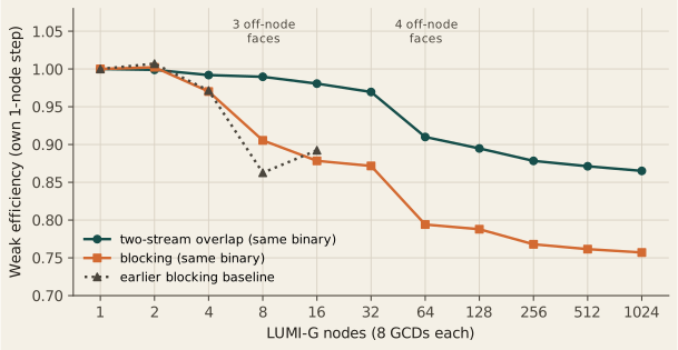
The earlier blocking baseline explains where the loss comes from. From one to sixteen nodes the halo phase grows from 0.206 to 0.313 ms, while the stencil and update kernels stay at 0.38 and 0.33 ms. That 0.107 ms growth matches the 0.110 ms growth of the whole step. Overlap hides most of that wait. It does not remove it: the remaining loss tracks the number of off-node faces per rank, which reaches four at 64 nodes, and then a small drift at fixed face count.
| Nodes | Off-node faces | Blocking (ms) | Overlap (ms) | Overlap efficiency |
|---|---|---|---|---|
| 1 | 0 | 0.910 | 0.859 | 1.00 |
| 32 | 3 | 1.044 | 0.886 | 0.97 |
| 64 | 4 | 1.146 | 0.944 | 0.91 |
| 256 | 4 | 1.185 | 0.978 | 0.88 |
| 1,024 | 4 | 1.202 | 0.993 | 0.87 |
Stencil order: wider halos, lower efficiency
Scaling A second campaign repeats the constant-\(256^3\) protocol for stencil orders 2, 4, 8, 12 and 20 on a different process-grid family, through 1,024 nodes. A higher order has a wider halo, so each step sends more bytes per face.
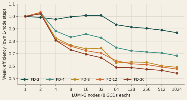
At 1,024 nodes weak efficiency is 0.869 for FD-2, 0.684 for FD-4, 0.590 for FD-8, 0.575 for FD-12 and 0.542 for FD-20. The higher orders lose most of that by 4 to 16 nodes, then decline slowly. At 1,024 nodes the halo wait that overlap cannot hide grows in the ratios 1.0, 1.9, 3.7, 6.0 and 9.9, against face sizes in the ratios 1, 2, 4, 6 and 10. The cost of order is communication.
Efficiency falls with order at most measured scales, but not all: at 64 nodes FD-12 (0.642) sits above FD-8 (0.626). This is a measured cost of halo width on this machine. It is not an accuracy ranking of the orders, and it did not change the production default.
A fixed 4096³ problem, 4 to 1,024 nodes
Scaling Strong scaling holds the global problem at \(4096^3\) cells, 68.7 billion, and adds nodes. Each cell of Figure 3 is the median of three allocations.
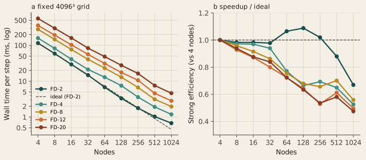
FD-2 goes from 115.649 ms per step on 4 nodes to 0.675 ms on 1,024 nodes, 171.3× for a 256× increase in hardware, an efficiency of 0.669. To 32 nodes the efficiency stays at 0.98. At 64 and 128 nodes it rises to 1.07 and 1.09: the owned brick shrinks to \(512^3\) and then \(512\times512\times256\), where a GCD works faster per cell. This is a local-brick effect, not better-than-ideal communication. From 256 nodes onward communication takes over.
The higher orders reach 134.4× (FD-4), 142.8× (FD-8), 126.8× (FD-12) and 121.4× (FD-20) at 1,024 nodes, efficiencies 0.474 to 0.558. Here FD-8 sits above FD-4, so strong-scaling efficiency is not monotone in order either.
Fixed grids on fewer GCDs
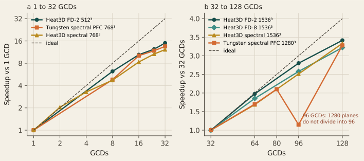
Scaling Smaller fixed problems show where a single application stops gaining from more GCDs.
| Workload | Grid | 1 GCD | 32 GCDs | Speedup |
|---|---|---|---|---|
| Heat3D FD-2 | \(512^3\) | 5.91 ms | 0.394 ms | 15.0× |
| Tungsten PFC (spectral) | \(768^3\) | 851 ms | 63 ms | 13.5× |
| Heat3D spectral | \(768^3\) | 416 ms | 34 ms | 12.2× |
With halo overlap the \(512^3\) step falls further, to 0.344 ms on 32 GCDs. Even so, a \(512^3\) grid is too small to keep scaling: each GCD’s brick becomes too thin.
At \(1536^3\), which divides evenly over 32, 64, 96 and 128 GCDs, the three heat-equation operators gain 3.2× to 3.4× from 32 to 128 GCDs: spectral 283 to 85 ms, FD-2 5.91 to 1.73 ms, FD-8 15.7 to 4.86 ms. Tungsten at \(1280^3\) gains 3.28× over the same range, but its 96-GCD run takes 258.67 ms, slower than 64 GCDs. 1280 planes do not divide into 96 slabs. Process count and decomposition are part of the execution design. The Tungsten article discusses this ladder with its model.
Distributed FFTs: weak scaling
Scaling Spectral methods transpose whole arrays, so their weak scaling is a different curve. Two constant-work series are measured.
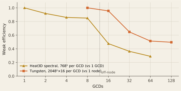
Heat3D spectral takes 416 ms on one GCD and 489 ms on eight GCDs of one node, 85% efficiency. The first step off the node, to 16 GCDs, costs the most: 873 ms, 48%. Eight nodes reach 1,434 ms, 29%. Tungsten, with smaller messages per step, keeps 49.6% at 16 nodes and a global \(2048^3\) grid. Neither series should be compared with finite-difference wall times: the operators and the local work differ.
Communication is the computation
At scale a spectral step is mostly data movement. These measurements ask how that movement is organised and how close it runs to the network. A separate halo-only timing, with no field update, is in Halo bandwidth. That page includes the contiguous face and a direct NVLink copy on the same H100 node.
Reshape protocols: no universal winner
Engineering HeFFTe can carry each global transpose with four MPI protocols. A tournament froze the binary, the layout and the physics and varied only the protocol, on two local workloads per GCD.
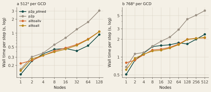
With \(512^3\) per GCD, p2p_plined is fastest from 32 to 128 nodes. With \(768^3\) per GCD the winner changes with scale: the collectives win at 4 to 64 nodes, p2p_plined at 128 and 256, and alltoallv at 512 nodes (2.108 s against 2.419 s). Plain p2p falls far behind at scale, 6.08 s at 512 nodes. A randomized follow-up at 124 to 528 nodes confirms that collectives beat plain p2p everywhere, while alltoall and alltoallv stay within 2% of each other: that pair is not ranked.
The best protocol depends on both scale and local workload. No node-count rule was justified, and the production default did not change.
Decomposition is a first-order variable
Engineering The same grid on the same ranks can run at very different speeds depending on how it is split.
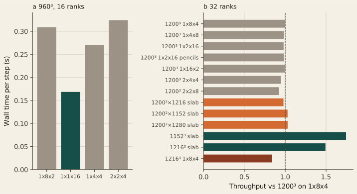
At \(960^3\) on 16 ranks a \(1\times1\times16\) slab takes 0.168 s per step and the \(1\times8\times2\) grid 0.309 s. At \(1200^3\) on 32 ranks, however, all seven legal grids sit between 0.420 and 0.455 s. Forcing a slab with nearby matched work (\(1200\times1200\times N_z\), \(N_z\) = 1152, 1216, 1280) gives 0.98 to 1.03 times the baseline throughput, while the cubic \(1152^3\) and \(1216^3\) slabs reach 1.74 and 1.49 times. Slab availability alone does not explain the slow \(1200^3\) case. That negative result led to the reshape fix in Section 4.
Close to the network
Engineering About 7.3 GB move per rank per step in the \(768^3\)-per-GCD transform plan. A tracing build measured the MPI time inside the solver and compared its byte rate with the OSU all-to-all benchmark at the same message size.
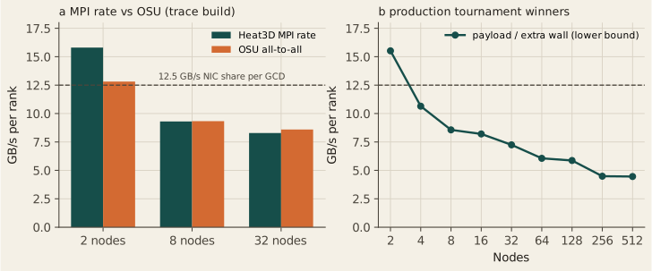
At 8 nodes the solver’s all-to-all moves 9.30 GB/s per rank and OSU 9.33 GB/s. At 32 nodes the figures are 8.29 and 8.59. The slowdown at these scales is MPI at the NIC, not a hidden local FFT problem. On one node the exchange runs over Infinity Fabric instead of the NIC, so the one-node rate (62 GB/s per rank) is not on the same scale. At 512 nodes the same 7.5 GB per rank moves at a lower bound of 4.5 GB/s per rank, in 0.92 MB messages.
Fewer transposes for derivatives
Experiment A gradient and part of a Hessian are usually taken with one forward and one backward 3D FFT per derivative, and each 3D FFT moves the whole field through every transpose. A derivative along one direction needs only a 1D transform along that direction. A standalone benchmark takes each derivative with 1D transforms in the pencil or slab layout where its directions are local, moves only the fields a later direction needs, and returns every result to the input layout. The baseline is HeFFTe 2.4.1 fft3d_r2c with the best of its reorder, reshape-protocol and batching options for each rank count, rocFFT and GPU-aware MPI.
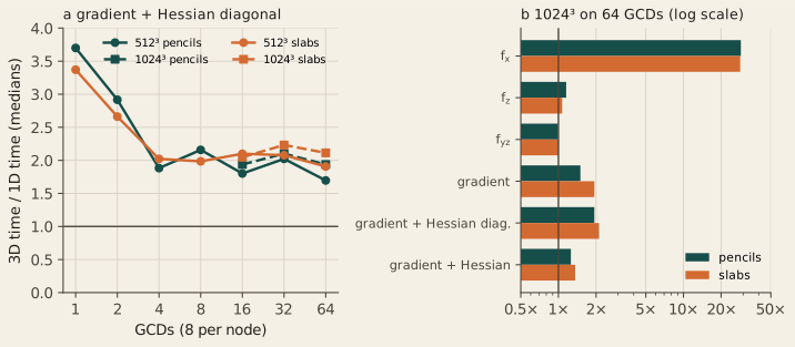
On 64 GCDs over 8 nodes the gradient with the Hessian diagonal takes 12.7 ms against 21.5 ms at \(512^3\) with pencils (1.70×) and 92.9 against 180.0 ms at \(1024^3\) (1.94×). Slabs give 1.91× and 2.11×. The saving comes from moving fewer fields: 6 instead of 14 with pencils, 3 instead of 7 with slabs. It is smaller than on one node because what remains is still communication. The reshapes are 87 to 92% of the 1D time on 64 GCDs.
The method does not help every derivative. A derivative along the input’s local direction, \(f_x\), needs no transpose and is 11 to 37 times faster on 8 GCDs or more. A single \(y\)–\(z\) mixed derivative moves almost as much data as the 3D route and takes 0.81 to 1.05 of its time. The method also holds 1.8 to 1.9 times the device memory for the full Hessian, against a 3D plan run one field at a time, because fields stay in several layouts. \(1024^3\) on 8 GCDs ran out of memory in the 1D tuning and has no result.
Every completed result matches the exact derivatives within \(64\,\epsilon\,n^p\), \(p\) the derivative order. The idea may be common practice in pseudo-spectral codes; no prior-art check has been made, and no novelty is claimed. A Laplacian already needs only one 3D transform pair, so OpenPFC’s Laplacian-type operators would not gain from it.
GPU-aware MPI
Engineering On one node, \(768^3\) on 8 GCDs, turning GPU-aware MPI off raises the spectral step from 75.9 to 503 ms, 6.6×, with an identical checksum. Host-staged transfers are not a production option. The ratio belongs to this control; it is not a factor for every application.
8,192 GCDs for FFTs: not possible on LUMI today
The \(768^3\)-per-GCD tournament was attempted on 1,024 nodes, 8,192 GCDs, four times between 3 and 9 October 2026. Every attempt aborted in the Slingshot fabric with No route to host before a timing profile was written. One suspect cabinet was excluded each time. Finite-difference jobs on the same node count complete. The admitted FFT curve ends at 512 nodes, and no 1,024-node FFT time is shown.
Performance engineering
These changes went into production because a measurement showed they helped. The failed attempts are part of the record.
Halo overlap: two failures, then a second stream
Engineering The blocking baseline in Section 2 showed halo time growing while the stencil stayed flat. Overlapping the two was the obvious idea, and the first two versions were not faster.
| Variant | Nodes | Overlap (ms) | Blocking (ms) | Decision |
|---|---|---|---|---|
| Six border launches | 2 | 0.945 | 0.907 | rejected |
| Six border launches | 4 | 0.950 | 0.937 | rejected |
| One fused border launch | 2 | 0.910 | 0.904 | rejected, neutral |
| One fused border launch | 4 | 0.915 | 1.001* | rejected, neutral |
| Interior on a second HIP stream | 2 | 0.860 | 0.908 | promoted |
| Interior on a second HIP stream | 4 | 0.866 | 0.938 | promoted |
With the interior kernel on the default stream, the GPU-aware MPI_Waitall did not progress while the kernel ran, and six thin border launches cost more than the wait they hid. Moving the interior kernel to a second HIP stream let the exchange progress: exposed halo wait fell from 0.419 to 0.241 ms. That version became the production default and is the overlap curve in Figure 1.
Minimum-reshape FFT layout
Engineering The slow \(1200^3\) case of Figure 7 traced to a rule in OpenPFC, not in HeFFTe. The old rule placed the transform’s complex output on a y-slab only when \(N_y\) divided evenly by the rank count; otherwise it kept an extra pencil-to-slab reshape. A new selector chooses the legal layout with the fewest reshapes.
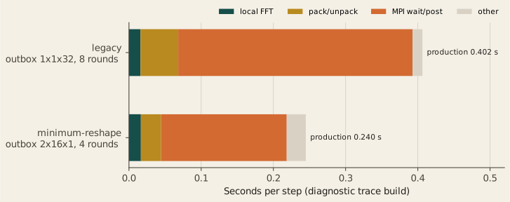
On the production build the step falls from 0.402 to 0.240 s, with the same spectral checksum. The tracing build shows why: all-to-all rounds per step fall from 8 to 4 and MPI time from 0.324 to 0.174 s, while the local FFT stays at 0.016 s. Grids that already had the short schedule keep it. This removes an avoidable reshape. It is a runtime layout fix, not a new FFT algorithm. Each arm is one allocation.
Decisions at a glance
| Episode | Outcome | Production effect |
|---|---|---|
| Early halo-overlap variants | rejected | blocking kept at the time |
| Two-stream halo overlap | promoted | overlap is the default |
| Slow \(1200^3\) FFT grid | slab hypothesis rejected | none |
| Minimum-reshape layout | promoted | new layout selector |
| HeFFTe protocol tournament | unresolved | default protocol unchanged |
| Finite-difference order | communication explains the loss | default order unchanged |
Acceleration
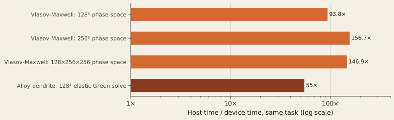
Acceleration These ratios compare a host run with a GPU run of the same task at the same size. They are not scaling results and do not transfer between applications.
Vlasov–Maxwell: ported by profile
A \(256^3\) phase-space step takes 1,036 ms on the host and 6.6 ms on one GCD, 156.7×; \(128^3\) reaches 93.8× and \(128\times256\times256\) 146.9×. The port followed the profile in two rounds. On the host the two velocity shifts and the moment reduction were 37%, 15% and 30% of the step. Porting those three took the step from 1.036 to 0.127 s and turned the profile over: the host spatial shift was then 77%, and the copies it forced another 19%. Only then was the shift moved to the GPU with hipFFT, which keeps the data resident for the whole step.
Two parts were measured and left on the host. The field solve costs 0.13 ms per step, 1.9% of the device step, about what its kernel launches would cost. A GPU-aware velocity halo would save a fraction of 0.02 ms. These device timings are capability measurements: the exact executable revision was not pinned beside each run.
On the host, a fixed \(128\times512\times512\) phase space scales from 27.73 s on 8 ranks to 5.11 s on 64 ranks, 5.43×, or 68% efficiency. The decomposition splits one velocity axis only, so the application refuses more than 85 ranks for this size rather than make a slab thinner than its halo.
Alloy dendrite: the elastic Green solve on the GPU
The \(128^3\) elastic solve takes 2,736 ms on the host path and 49.6 ms on the HIP device path, about 55×, with the same eight iterations on both. The timed device path makes no host round trips, so the ratio measures the ported solve, not a host fallback. This is an implementation result. It does not change the physical dendrite findings.
Raw step time is not method cost
Method cost On a common grid the spectral operator is far slower per step than a finite-difference stencil. That is only half of a cost comparison.
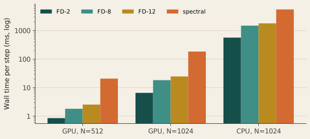
| Operator | GPU, \(N=512\) | GPU, \(N=1024\) | CPU, \(N=1024\) |
|---|---|---|---|
| FD-2 | 0.856 ms | 6.572 ms | 569 ms |
| FD-8 | 1.821 ms | 18.319 ms | 1,492 ms |
| FD-12 | 2.553 ms | 24.701 ms | 1,796 ms |
| Spectral | 20.767 ms | 184.386 ms | 5,525 ms |
A spectral operator resolves more of the spectrum per grid point, so a fair comparison asks what each operator costs to reach the same accuracy. For a periodic Gaussian benchmark, a validated error model gives the grid each operator needs; the measured step costs then give the price.
| Target error | GPU node | CPU node |
|---|---|---|
| \(10^{-2}\) | FD-2 cheaper: 0.051× spectral | FD-2 cheaper: 0.17× spectral |
| \(10^{-8}\) | spectral cheaper: best FD-12 costs 3.1× | spectral cheaper: FD-12 costs 8.8× |
At a loose tolerance finite differences win; at a tight one the spectral operator wins, on both nodes. The three-repeat GPU matrix at \(N=512\) and \(1024\) keeps both conclusions (FD-2 at 0.067× and 0.058×; best FD-12 at 3.3× and 3.6×). This is a cost model built on measured step times, not an end-to-end solver race, and it covers this benchmark family. Equal-grid wall time can rank discretizations the wrong way.
Execution envelope
| Run | Nodes | GCDs | Grid | Result | Status |
|---|---|---|---|---|---|
| Heat3D FD-2 weak, overlap | 1,024 | 8,192 | \(2048^2\times32768\) | 0.993 ms/step | admitted |
| Heat3D FD strong, orders 2–20 | 1,024 | 8,192 | \(4096^3\) | 0.675 ms/step (FD-2) | admitted |
| HeFFTe tournament | 512 | 4,096 | \(768^2\times3145728\) | 2.108 s/step | admitted |
| HeFFTe tournament | 1,024 | 8,192 | \(768^2\times6291456\) | no timing | fabric abort |
| Tungsten slab weak | 16 | 128 | \(2048^3\) | 412.39 ms/step | admitted |
| Tungsten cubic | 60 | 480 | \(3000^3\) | 0.856 s/step | execution only |
The \(3000^3\) Tungsten run shows that the application executes at that size. Its cubic weak-scaling family mixes process-grid families and carries stale source provenance, so it is not a scaling endpoint. On a single GCD, Tungsten steps \(256^3\) in 20 ms and \(768^3\) in 847 ms.
Boundaries
What these results show
- How the finite-difference and spectral paths behave on LUMI-G up to 1,024 nodes, each against its own baseline.
- Where time goes: halo faces for stencils, all-to-all transposes for FFTs.
- Which runtime changes helped, which did not, and by how much.
- Host-to-GPU ratios for two named computations.
- That equal-grid step time and equal-accuracy cost can disagree.
What they do not show
- A single OpenPFC speedup. Workloads, baselines and machines differ.
- An OpenPFC speedup from one-direction derivatives. That benchmark runs outside the runtime.
- A comparison between weak and strong scaling, or between scaling and acceleration.
- One application’s ratio applied to another.
- Today’s
master: runs used recorded September–October 2026 revisions. - Kobayashi GPU scaling. A two-point H100 workflow exists; it is not a scaling curve.
- Wall-clock speedups for inverse homogenization. Its reductions are solve counts.
- Further LUMI runs still under review: multi-GCD Vlasov device timings, a \(1024^3\) Taylor–Green step-time window and production-size solidification runs.
Data and methods
Each figure is drawn from a compact table frozen from the reviewed measurement records. Timing is the median per-step wall time after warm-up steps, synchronised across ranks, with one MPI rank per MI250X GCD. Each table states its own protocol in its header.
Weak scaling · blocking baseline · stencil order · exposed wait · 4096³ strong · fixed grids · FFT weak · Tungsten one GCD · protocols · protocol follow-up · decomposition · reshape layout · payload · OSU · derivatives · halo variants · acceleration · Vlasov host · method cost · equal accuracy · envelope
The OpenPFC documentation explains the campaigns and their analysis: GPU scaling on LUMI, finite-difference weak scaling, stencil order, protocol tournament, protocol follow-up, bandwidth calibration, Vlasov GPU port and method cost.