Polynomial methods / Learn by experiment
An integral is a boundary-value problem
Recover four definite integrals by solving for an antiderivative with OpenPFC GMRES.
Download runnable lesson (.zip)
Includes the model, inputs, required headers and a short run guide.
An integral can be computed without introducing quadrature weights first. Program 30 of Trefethen (2000) solves the initial-value problem
\[ \begin{gathered} v'(x)=f(x), \\ v(-1)=0, \\ I=v(1). \end{gathered} \tag{1}\]
We use the same Chebyshev collocation experiment for the four functions from the regularity lesson, replacing the book’s explicit matrix inverse with OpenPFC’s GMRES solver.
Remove the known endpoint
The nodes run from \(x_0=1\) to \(x_N=-1\). The last value of \(v\) is known, so it is removed from the unknown vector. We impose \(v'=f\) at the first \(N\) nodes and solve
\[D_{0:N-1,\,0:N-1}\,v_{0:N-1}=f_{0:N-1}. \tag{2}\]
The desired integral is the first component, \(v_0\). There is no sign flip: the order of stored nodes does not change the direction of the integral.
for (int n = 1; n <= maximum; ++n) {
  const auto x = polynomial::nodes(n);
  const auto d = polynomial::differentiation(x);
  polynomial::Matrix a(n, polynomial::Vector(n));
  for (int i = 0; i < n; ++i)
    for (int j = 0; j < n; ++j) a[i][j] = d[i][j];
  for (int type = 0; type < 4; ++type) {
    polynomial::Vector f;
    for (int j = 0; j < n; ++j)
      f.push_back(polynomial::profile(type, x[j]).value);
    const auto antiderivative = polynomial::solve(a, f);
    const double exact = polynomial::profile(type, 0).integral;
    output << n << ',' << type << ',' << antiderivative[0] << ',' << exact << ','
           << std::abs(antiderivative[0] - exact) << '\n';
  }
}
Give the linear solver an operator
OpenPFC’s solver accepts an action \(w=Av\) and vector operations. This small example stores a dense matrix; the same solver contract also admits an operator that never forms a matrix. Each equation is scaled by its largest coefficient before solving. The stopping norm therefore belongs to the scaled equations, and the tests separately check the physical integral.
inline Vector solve(Matrix a, Vector b) {
  // Row scaling changes the residual norm, not the solution.
  for (std::size_t i = 0; i < a.size(); ++i) {
    double scale = 0;
    for (double entry : a[i]) scale = std::max(scale, std::abs(entry));
    if (!(scale > 0)) throw std::runtime_error("Empty equation");
    for (double &entry : a[i]) entry /= scale;
    b[i] /= scale;
  }
  pfc::solvers::VectorOperations<> ops;
  pfc::solvers::KrylovControls controls;
  controls.relative_tolerance = 1e-12;
  controls.absolute_tolerance = 1e-14;
  controls.restart = static_cast<int>(b.size());
  controls.maximum_iterations = 4 * controls.restart;
  Vector u(b.size());
  const auto result = pfc::solvers::gmres(
      ops, [&](const auto &v, auto &w) { w = polynomial::apply(a, v); }, b, u,
      controls);
  if (!result.converged()) throw std::runtime_error("GMRES did not converge");
  return u;
}
We use GMRES because this collocation matrix is not symmetric positive definite. Choosing CG merely because the continuous problem is simple would violate CG’s algebraic assumptions. VectorOperations uses local arithmetic here; these complete-domain reference models run on one process.
Separate solver error from approximation error
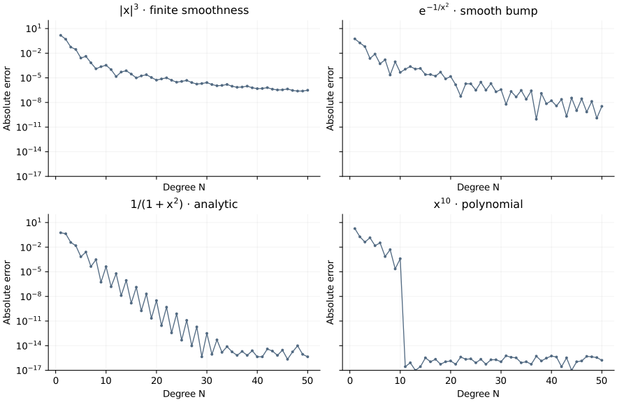
openpfc run model.cpp input.json --source-root .. --launcher=noneThe exact integrals, in profile order, are \(1/2\), \(2[e^{-1}-\sqrt\pi\operatorname{erfc}(1)]\), \(\pi/2\) and \(2/11\). results/integrals.csv records the computed integral and its error for every degree up to n, initially 50.
The derivative of a degree-\(N\) antiderivative has degree at most \(N-1\). Thus \(x^{10}\) needs \(N\ge11\) for exact integration by this construction, one degree later than its exact differentiation in the previous lesson. The tests check those exact cases, the analytic integral, and the complete low-degree systems against independent polynomial antiderivatives. Tightening a Krylov tolerance cannot repair a poorly resolved source. For the logarithmic plot, zero errors are placed at the \(10^{-17}\) display floor; the CSV retains zero when the rounded integral equals the reference.
The complete C++ model and starting input are available with this lesson. It also uses the shared collocation.hpp; keep its relative location when saving the files.