OpenPFC / One equation, another timestep
An implicit solve can be a division
Fourier modes diagonalize the Laplacian. That makes an implicit heat step almost as short as an explicit one.
Download runnable lesson (.zip)
Includes the model, inputs, required headers and a short run guide.
Return to the common heat problem:
\[ \begin{aligned} u_t&=D\Delta u,\\ u(\mathbf x,0)&=1+.2\cos x\cos y\cos z. \end{aligned} \tag{1}\]
The original 04_diffusion_model used a Gaussian and an approximate value of pi in its grid. This refactoring keeps its implicit spectral method, uses physical wave numbers from the native iterator, and joins the same controlled mode comparison as the other heat lessons.
Move the new Laplacian to the left
Backward Euler evaluates diffusion at the new time level:
\[ (I-D\Delta t\Delta)u^{m+1}=u^m. \tag{2}\]
Since \(\widehat{\Delta u}=-|\mathbf k|^2\hat u\), each Fourier coefficient solves one scalar equation:
\[ \hat u^{m+1}_{\mathbf k}= \frac{\hat u^m_{\mathbf k}}{1+D\Delta t|\mathbf k|^2}. \tag{3}\]
std::vector<std::complex<double>> modes(fft.size_outbox());
std::vector<double> denominator(modes.size());
pfc::fft::kspace::for_each_kpoint(
    fft.get_outbox_bounds(), heat::domain(p),
    [&](std::size_t i, double kx, double ky, double kz, int, int, int) {
      denominator[i] = 1 + p.dt * p.diffusivity * (kx * kx + ky * ky + kz * kz);
    });
auto diagnostics = heat::open_diagnostics(comm.rank());
heat::observe(u, p, 0, diagnostics, comm.rank());
for (int step = 1; step <= p.steps; ++step) {
  fft.forward(u.vec(), modes);
  for (std::size_t i = 0; i < modes.size(); ++i) modes[i] /= denominator[i];
  fft.backward(modes, u.vec());
  heat::observe(u, p, step * p.dt, diagnostics, comm.rank());
}
The multiplier never exceeds one for positive \(D\) and \(\Delta t\). Thus the linear heat discretization has no explicit-Euler stability limit. It still has first-order time error. Stability regions and spectral diagonalization are discussed in Trefethen (2000).
Predict the complete answer
For this initial cosine product, \(|\mathbf k|^2=3\). After \(m\) steps, the amplitude is \(.2(1+3D\Delta t)^{-m}\) rather than \(.2e^{-3Dm\Delta t}\). Backward Euler therefore decays this mode too slowly at a fixed physical time. The zero mode stays unchanged, so the mean remains one.
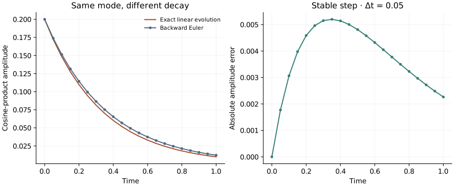
Use a stable step, then ask whether it is accurate
openpfc run model.cpp input.json --source-root .. --launcher=noneDouble dt and halve steps to keep the same end time. The solution remains linearly stable while its error grows. Compare with forward Euler and the exact linear propagator. The tests compare all physical samples with the discrete amplitude on one and two ranks, rather than checking just the field maximum.
Keep the model, input and common heat helper together. Complete fields and diagnostics are written under the run’s results/ directory.