Lesson 02 / Heat flow
Heat flow from neighbouring values
A warmer point gives heat to its neighbours. Can a few lines of C++ preserve that simple picture?
Download runnable lesson (.zip)
Includes the model, inputs, required headers and a short run guide.
The heat equation smooths temperature differences. A periodic box makes the bookkeeping especially revealing: heat cannot leave through an outer boundary, so the spatial mean must remain constant. A single cosine mode also gives us an exact decay rate. We can check conservation and accuracy without guessing what a plausible field should look like.
The separated-halo lesson studies the communication buffers while keeping the same physical problem.
One problem, three methods
Let \(\Omega=[0,2\pi)^3\) be periodic in every direction, with dimensionless coordinates and temperature. For constant diffusivity \(D>0\),
\[ \begin{gathered} \partial_t u=D\Delta u, \\ u(\mathbf{x},0)=1+0.2\cos x\cos y\cos z. \end{gathered} \tag{1}\]
Each second derivative of the cosine product is its negative, so
\[ u(\mathbf{x},t)=1+0.2e^{-3Dt}\cos x\cos y\cos z. \tag{2}\]
The spatial mean is one. The root-mean-square fluctuation about that mean is \(0.2e^{-3Dt}/\sqrt8\). Both identities follow directly from the mode; they are stronger checks than a decreasing maximum alone.
The Fourier and exponential lessons use precisely this problem. The shared lesson.hpp owns input validation and diagnostics; each model.cpp owns its numerical method.
Turn curvature into a stencil
On a uniform grid with \(h=2\pi/N\), approximate the Laplacian by
\[ (\Delta_hu)_{ijk}=\frac{ u_{i+1,j,k}+u_{i-1,j,k}+u_{i,j+1,k}+u_{i,j-1,k} +u_{i,j,k+1}+u_{i,j,k-1}-6u_{ijk}}{h^2}. \tag{3}\]
Opposite fluxes cancel when summed over the periodic grid. Consequently, forward Euler preserves the discrete mean, up to roundoff:
\[ u^{n+1}=u^n+\Delta t\,D\Delta_hu^n. \tag{4}\]
For \(r=D\Delta t/h^2\le1/6\), Equation 4 is a weighted average: the centre has weight \(1-6r\), and each neighbour has weight \(r\). These weights are nonnegative and sum to one. This gives an intuitive stability condition; the most negative stencil eigenvalue, \(-12/h^2\), gives the same forward-Euler limit. Fixed-order differences and spectral differentiation are introduced together in Trefethen (2000), chapter 1 and program 5.
Let the code show the equation
Decompose the periodic domain, allocate a field with one layer of ghost cells, and initialise its owned values:
const auto decomp = pfc::decomposition::create(heat::domain(p), comm.size());
auto u = pfc::data::field_from_subdomain<double>(decomp, comm.rank(), 1);
pfc::comm::HaloExchange<pfc::HostSpace, double> halo(u, decomp, comm.rank(),
                                                     comm);
u.apply([&](double x, double y, double z) {
  return heat::exact(x, y, z, 0.0, p.diffusivity);
});
auto gradient = pfc::field::create<heat::Derivatives>(u, 2);
auto du = pfc::data::field_from_subdomain<double>(decomp, comm.rank(), 1);
The 2 in the gradient factory selects second-order central differences. The derivative aggregate asks for xx, yy, and zz; the model does not request or calculate first derivatives. Now Equation 4 becomes:
for (int step = 1; step <= p.steps; ++step) {
  halo.exchange();
  u.for_each_owned([&](int i, int j, int k) {
    const auto g = gradient(i, j, k);
    du(i, j, k) = p.diffusivity * (g.xx + g.yy + g.zz);
  });
  u += p.dt * du;
  heat::observe(u, p, step * p.dt, diagnostics, comm.rank());
}
halo.exchange refreshes neighbouring values in the padded ghost cells. for_each_owned evaluates the right-hand side at every owned cell before u changes. du has the same padded layout as u, so the field update uses matching storage indices. u += p.dt * du is an array update through OpenPFC’s field operators. This ordering matters: overwriting one cell before calculating its neighbour’s derivative would define a different method.
Predict the answer before running
For our cosine product, Equation 3 has the exact discrete eigenvalue
\[ \begin{gathered} \lambda_h=-\frac{12}{h^2}\sin^2(h/2), \\ A_n=0.2(1+D\Delta t\lambda_h)^n. \end{gathered} \tag{5}\]
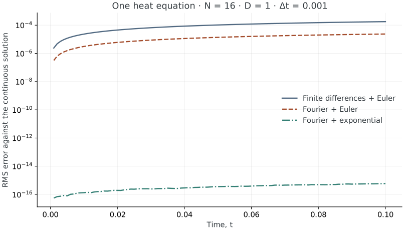
Thus the complete computed field should equal \(1+A_n\cos x_i\cos y_j\cos z_k\), within roundoff. Compare it with Equation 2 to measure the combined spatial and temporal error. A small error can reflect cancellation between these two contributions; one fine-looking answer is not a convergence study.
Run and experiment
From examples/heat/finite-differences:
openpfc run model.cpp input.json --source-root .. --launcher=none--source-root .. includes the shared ../lesson.hpp in the preserved source snapshot. The input remains input.json, and the implementation is model.cpp.
The printed attempt directory contains results/diagnostics.csv and one results/field_rank_<rank>.csv per rank. Diagnostics are global: mean should stay near one, rms_fluctuation should decrease, and rms_error compares every cell with Equation 2. The field CSV records physical coordinates, computed temperature, and the exact value.
Try halving dt and doubling steps, keeping the final time fixed. Then double n, divide dt by four, and multiply steps by four. Explain why both changes affect the error. Finally, set dt above \(h^2/(6D)\): the program should reject the input before advancing the field.
To compare MPI decompositions, invoke the CLI once with --ranks=2 --launcher=mpirun in place of --launcher=none. Compare the global diagnostics; expect small floating-point differences, not necessarily identical CSV bytes.
Verification and scope
The example checks compare every computed cell against Equation 5, verify the reported continuum error, conservation, and decay, and reject unstable inputs. One- and two-rank runs check the communication boundary. These are periodic constant-coefficient teaching cases, not a model of heat loss through a material surface.
Next: keep the physics and change the spatial derivative.
The complete C++ model and starting input are available with this lesson. It also uses the shared lesson.hpp; keep its relative location when saving the files.