Lesson 03 / Fourier heat flow
Same heat, different derivative
What if the spatial derivative is already exact for our wave, but the answer still has an error?
Download runnable lesson (.zip)
Includes the model, inputs, required headers and a short run guide.
In the previous lesson, a finite stencil approximated curvature. Here we change that one numerical choice. The periodic domain, initial condition, physical right-hand side, and Euler update remain the same. This refactors the former 20_explicit_stepper_spectral.cpp around an independently checkable field.
A heat equation in Fourier space
For the periodic problem on \([0,2\pi)^3\),
\[ \begin{gathered} \partial_t u=D\Delta u, \\ u(\mathbf{x},0)=1+0.2\cos x\cos y\cos z, \end{gathered} \tag{1}\]
write a trigonometric interpolant \(u_N(\mathbf{x})=\sum_{\mathbf{k}}\widehat u_{\mathbf{k}} e^{i\mathbf{k}\cdot\mathbf{x}}\). Its Laplacian is
\[ \widehat{\Delta u}_{\mathbf{k}}=-|\mathbf{k}|^2\widehat u_{\mathbf{k}}. \tag{2}\]
Differentiation becomes multiplication by a known symbol. The constant mode has \(\mathbf{k}=0\) and remains unchanged. Each nonconstant mode in our initial condition has \(|\mathbf{k}|^2=3\).
These modes are represented exactly on our grid. Fourier differentiation therefore introduces no truncation error for this particular field, apart from roundoff. That property belongs to a resolved trigonometric mode; it does not mean the method exactly differentiates every smooth function at a finite resolution (Trefethen 2000, programs 1 and 5).
Change the stack, keep the equation
pfc::sim::stacks::SpectralCPUStack stack(heat::domain(p), comm.rank(),
                                         comm.size());
auto &u = stack.u();
u.apply([&](double x, double y, double z) {
  return heat::exact(x, y, z, 0.0, p.diffusivity);
});
auto du = stack.du<heat::Derivatives>();
Compare the initialisation with the FD lesson. SpectralCPUStack sizes the field to the FFT’s local real-space box. Its evaluator transforms the field and applies Equation 2 for the requested second derivatives. There is no face-halo exchange in this implementation.
The physical update stays the same:
for (int step = 1; step <= p.steps; ++step) {
  du.apply([&](const heat::Derivatives &g) {
    return p.diffusivity * (g.xx + g.yy + g.zz);
  });
  u += p.dt * du;
  heat::observe(u, p, step * p.dt, diagnostics, comm.rank());
}
The physics still reads \(D(u_{xx}+u_{yy}+u_{zz})\). Keeping that expression visible makes the boundary between physical law and numerical method easy to inspect.
Why is there still an error?
The exact mode amplitude is \(A(t)=0.2e^{-3Dt}\). Euler instead gives
\[ A_n=0.2(1-3D\Delta t)^n. \tag{3}\]
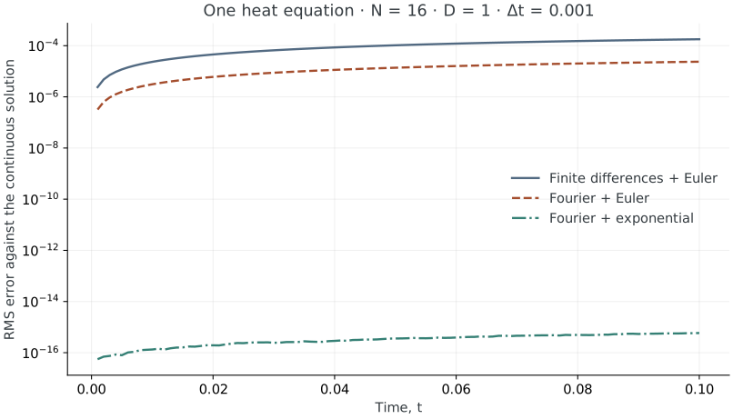
At a fixed final time, this is a first-order approximation in \(\Delta t\). Increasing \(N\) cannot fix it. Halving \(\Delta t\) should roughly halve the error once the asymptotic regime is reached.
Stability also belongs to the time integrator. On an even grid the most negative Laplacian symbol is \(-3(\pi/h)^2\). Euler requires
\[ \Delta t\le\frac{2h^2}{3D\pi^2}. \tag{4}\]
This bound is stricter than the second-order FD bound. Although our initial field contains only low modes, the executable enforces the bound for the complete represented spectrum, including perturbations introduced by roundoff.
Try the experiment
From examples/heat/fourier:
openpfc run model.cpp input.json --source-root .. --launcher=noneInspect the printed attempt’s results/diagnostics.csv and final field CSVs. The columns and exact solution are the same as in the FD lesson. The source is model.cpp; parameters are in input.json.
First change n from 16 to 32, keeping dt and steps fixed. The continuum error should be almost unchanged. Then return to n=16, halve dt, and double steps: the final time stays fixed while the temporal error decreases.
A useful wrong expectation is that a finer spectral grid permits a larger explicit timestep. Try n=64 with the original dt=0.001. The input should be rejected by Equation 4. Explain why resolving shorter waves makes this explicit method more restrictive.
Verification and scope
The example checks reconstruct the entire field from Equation 3, independently of OpenPFC’s FFT routines. They also check the zero mode, RMS decay, continuum error, invalid inputs, and one versus two MPI ranks. This chapter covers a periodic linear equation on the CPU. It introduces neither nonlinear dealiasing nor nonperiodic boundary conditions.
The next lesson removes Euler’s approximation by solving each linear Fourier-mode equation analytically.
The complete C++ model and starting input are available with this lesson. It also uses the shared lesson.hpp; keep its relative location when saving the files.