Lesson 04 / Exponential evolution
Let each wave decay exactly
Once a PDE becomes independent scalar ODEs, why approximate an evolution we can solve?
Download runnable lesson (.zip)
Includes the model, inputs, required headers and a short run guide.
Fourier differentiation made the spatial operator exact for our cosine mode, but forward Euler left a time error. Constant diffusivity gives us another option: solve the equation of each Fourier coefficient analytically. The resulting implementation is a transform, a multiplication, and an inverse transform.
The forward/multiply/backward pattern keeps the mathematical update visible. Compare its exact linear multiplier with the implicit approximation in backward-Euler heat.
Solve the coefficient equation
For \(\partial_tu=D\Delta u\) on the periodic box, every represented mode satisfies
\[ \frac{d\widehat u_{\mathbf{k}}}{dt} =-D|\mathbf{k}|^2\widehat u_{\mathbf{k}}. \tag{1}\]
Separation of variables gives
\[ \widehat u_{\mathbf{k}}(t+\Delta t) =e^{-D|\mathbf{k}|^2\Delta t}\widehat u_{\mathbf{k}}(t). \tag{2}\]
The multiplier lies in \([0,1]\) for \(D,\Delta t>0\). At \(\mathbf{k}=0\) it is one, preserving the mean. Unlike Euler’s multiplier \(1-D|\mathbf{k}|^2\Delta t\), it cannot amplify a high-frequency mode.
For \(u(\mathbf{x},0)=1+0.2\cos x\cos y\cos z\), Equation 2 gives the same \(e^{-3Dt}\) decay as the continuous solution. This special initial condition is fully represented by the Fourier grid, so both spatial and temporal truncation errors vanish; roundoff remains.
Build the propagator once
The FFT’s real-space and Fourier-space decompositions can differ. Use the Fourier outbox, rather than assuming a local index is a global wavenumber:
std::vector<std::complex<double>> spectrum(fft.size_outbox());
std::vector<double> decay(fft.size_outbox());
pfc::fft::kspace::for_each_kpoint(
    fft.get_outbox_bounds(), heat::domain(p),
    [&](std::size_t i, double kx, double ky, double kz, int, int, int) {
      decay[i] = std::exp(-p.diffusivity * (kx * kx + ky * ky + kz * kz) * p.dt);
    });
for_each_kpoint supplies physical wavenumbers, including spacing and frequency ordering. The vectors contain only the modes owned by this rank. The propagator depends on the fixed timestep and diffusivity, so we calculate it once.
Now advance the field:
for (int step = 1; step <= p.steps; ++step) {
  fft.forward(u.vec(), spectrum);
  for (std::size_t i = 0; i < spectrum.size(); ++i) spectrum[i] *= decay[i];
  fft.backward(spectrum, u.vec());
  heat::observe(u, p, step * p.dt, diagnostics, comm.rank());
}
OpenPFC’s inverse FFT already supplies the normalization needed for a forward/backward round trip. Dividing by the global cell count again would destroy the mean: the conservation check would catch that mistake.
Compare three answers to one problem
| Method | Spatial action | One-step mode multiplier |
|---|---|---|
| FD + Euler | Second-order periodic stencil | \(1+D\Delta t\lambda_h\) |
| Fourier + Euler | Exact symbol on represented modes | \(1-D\Delta t|\mathbf{k}|^2\) |
| Fourier + exponential | Exact symbol on represented modes | \(e^{-D\Delta t|\mathbf{k}|^2}\) |
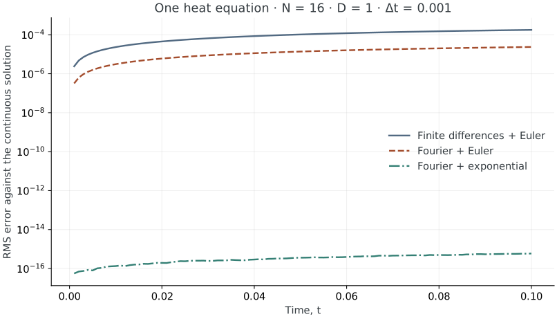
The existing backward-Euler diffusion example would use \(1/(1+D\Delta t|\mathbf{k}|^2)\). It is stable for linear diffusion but still has a temporal truncation error. Stability and exact integration are different properties.
Run it and test the idea
From examples/heat/exponential:
openpfc run model.cpp input.json --source-root .. --launcher=noneThe source is model.cpp, with input.json for parameters. As before, inspect results/diagnostics.csv and the final rank fields inside the attempt directory printed by the CLI.
Change to dt=0.1 and steps=1. This advances to the same final time as 100 steps of size 0.001, with a result still close to the exact solution. Compare their errors: taking more FFT round trips can accumulate more roundoff. An exact mathematical propagator does not make repeated floating-point computation exact.
As a deliberate counterexample, replace the exponential multiplier by \(1-D|\mathbf{k}|^2\Delta t\) and keep the large timestep. Predict which high-frequency modes amplify. The executable’s exponential path has no Euler stability guard, so this edited experiment needs its own stability analysis.
Where exact propagation ends
Variable diffusivity couples modes. Nonlinear terms such as \(u^3\) do too. Applying Equation 2 to the linear part alone does not integrate the whole nonlinear PDE exactly. Exponential time-differencing methods extend the idea by approximating the remaining contribution; Cox and Matthews develop higher-order schemes for stiff systems (Cox and Matthews 2002). That is the bridge to OpenPFC’s existing nonlinear spectral and ETD examples, rather than a claim that this short program implements a general ETD solver.
The numerical checks compare every cell with the independent cosine-mode solution, verify mean preservation and decay, and run on one and two ranks. General initial data still have Fourier truncation error; no nonperiodic or variable-coefficient case is qualified by these checks.
The complete C++ model and starting input are available with this lesson. It also uses the shared lesson.hpp; keep its relative location when saving the files.