Lesson 01 / Differentiation
How accurately can we differentiate?
A local stencil and a global trigonometric interpolant look at the same samples. How much can each one learn?
Download runnable lesson (.zip)
Includes the model, inputs, required headers and a short run guide.
Suppose all we know about a function is its value at equally spaced points. We can estimate a derivative from nearby values, or fit a periodic wave through every sample and differentiate that wave. Both are approximations. For a smooth periodic function, their errors behave very differently.
This experiment revisits the question in programs 1 and 5 of Trefethen (2000), using OpenPFC’s finite-difference and Fourier evaluators. The C++ implementation and explanation are independent; we reproduce the smooth-function comparison, rather than every experiment in those programs.
A derivative we already know
On the periodic interval \([0,2\pi)\), let
\[ \begin{gathered} u(x)=e^{\sin x}, \\ u'(x)=\cos x\,e^{\sin x}. \end{gathered} \tag{1}\]
Use \(N\) points \(x_j=jh\), with \(h=2\pi/N\). The point \(2\pi\) is the same periodic point as zero, so it is not stored twice. Our error is measured at the grid points:
\[ E_N=\max_j\left| (D_Nu)_j-u'(x_j)\right|. \tag{2}\]
The exact expression in Equation 1 supplies an independent reference. No PDE or time integrator can obscure the spatial approximation here.
Nearby values or Fourier modes?
The centred second- and fourth-order formulas are
\[ \begin{gathered} (D_2u)_j=\frac{u_{j+1}-u_{j-1}}{2h}, \\ (D_4u)_j=\frac{-u_{j+2}+8u_{j+1}-8u_{j-1}+u_{j-2}}{12h}. \end{gathered} \tag{3}\]
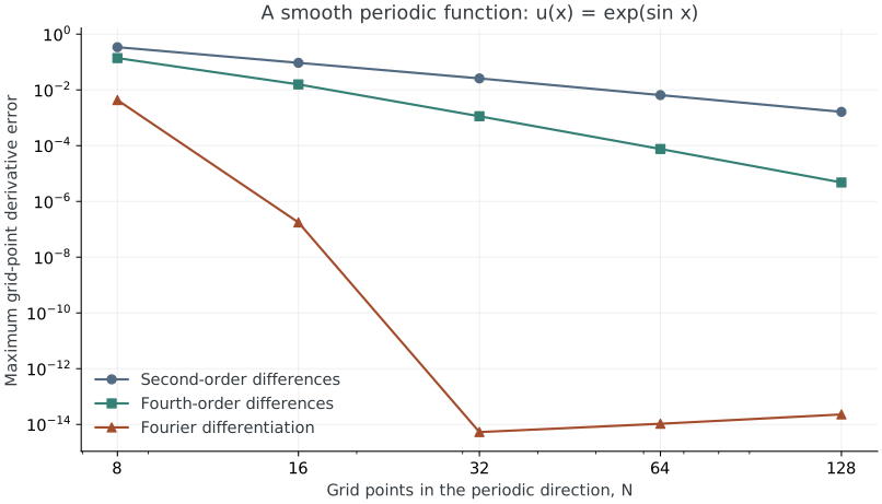
Taylor expansion cancels the lower-order error terms. For sufficiently smooth \(u\), the remaining errors scale like \(h^2\) and \(h^4\). Doubling \(N\) should therefore reduce the errors by approximately four and sixteen once the leading term dominates.
Fourier differentiation instead constructs the trigonometric interpolant \(u_N(x)=\sum_k\widehat u_k e^{ikx}\) and uses
\[ u_N'(x)=\sum_k ik\widehat u_k e^{ikx}. \tag{4}\]
OpenPFC evaluates Equation 4 with FFTs. For this analytic periodic function, the approximation error falls much faster than either fixed stencil’s algebraic rate, until floating-point roundoff becomes visible. Spectral accuracy depends on smoothness and periodic compatibility; it is not a promise for arbitrary sampled data (Trefethen 2000, programs 1 and 5).
Express the calculation in C++
Our requested derivative is just struct Derivative { double x{}; };. The evaluator calculates only that derivative. The same error calculation works with both derivative evaluators:
template <class Evaluator>
double derivative_error(const pfc::data::Field<double> &u, Evaluator &derivative) {
  derivative.prepare();
  double local_error = 0.0;
  u.for_each_owned([&](int i, int j, int k) {
    const double x = u.coords(i, j, k)[0];
    const double exact = exact_derivative(x);
    local_error = std::max(local_error, std::abs(derivative(i, j, k).x - exact));
  });
  double error = 0.0;
  MPI_Allreduce(&local_error, &error, 1, MPI_DOUBLE, MPI_MAX, MPI_COMM_WORLD);
  return error;
}
u.apply receives physical coordinates, including the global offset of each MPI subdomain. The final reduction computes the maximum over all ranks. The small \(N\times8\times8\) box repeats the same function in the transverse directions; it lets us use the usual three-dimensional stack without changing this one-dimensional mathematical problem.
Here is the complete comparison loop:
for (int n : sizes) {
  const double h = 2.0 * std::numbers::pi / n;
  const auto domain = pfc::domain::create(pfc::GridSize{{n, 8, 8}},
                                          pfc::PhysicalOrigin{{0.0, 0.0, 0.0}},
                                          pfc::GridSpacing{{h, 1.0, 1.0}});
  const auto decomp = pfc::decomposition::create(domain, comm.size());
  auto u = pfc::data::field_from_subdomain<double>(decomp, comm.rank(), 2);
  pfc::comm::HaloExchange<pfc::HostSpace, double> halo(u, decomp, comm.rank(),
                                                       comm);
  u.apply([](double x, double, double) { return value(x); });
  halo.exchange();
  auto fd2 = pfc::field::create<Derivative>(u, 2);
  auto fd4 = pfc::field::create<Derivative>(u, 4);
  pfc::sim::stacks::SpectralCPUStack fourier(domain, comm.rank(), comm.size());
  fourier.u().apply([](double x, double, double) { return value(x); });
  auto spectral = pfc::field::create<Derivative>(fourier.u(), fourier.fft());
  const double e2 = derivative_error(u, fd2);
  const double e4 = derivative_error(u, fd4);
  const double ef = derivative_error(fourier.u(), spectral);
  if (comm.rank() == 0) {
    file << n << ',' << e2 << ',' << e4 << ',' << ef << '\n';
    std::cout << n << "  " << std::scientific << e2 << "  " << e4 << "  " << ef
              << '\n';
  }
}
The finite-difference field has two layers of padding, enough for the fourth-order stencil. halo.exchange() fills those ghost cells before either FD evaluator reads them. SpectralCPUStack uses distributed FFTs. Neither changes the exact reference or the definition of error.
Run it, then change it
From this lesson’s directory, after installing the SDK:
openpfc run model.cpp input.json --launcher=noneThe printed attempt directory contains results/convergence.csv, with columns n,fd2,fd4,fourier. Its values supply Figure 1; the plotting command is in the examples authoring guide. The source is model.cpp and the editable input is input.json.
To extend the fourth-order comparison to the original program 1 resolutions, 8, 16, …, 4096, use the supplied preset:
openpfc run model.cpp trefethen-p1.json --launcher=noneThe second-order and FFT columns are additional comparisons. The larger grid does not change the mathematical interval; its spacing remains \(2\pi/N\).
Try sizes: [16, 32, 64, 128, 256] in the JSON file, retaining JSON’s quotes around "sizes". Predict the last two error ratios before looking at them. The FD ratios should approach four and sixteen. The Fourier errors should stop improving once roundoff dominates; do not fit a convergence rate to that plateau.
Then change value to \(\sin(3x)\) and exact_derivative to \(3\cos(3x)\). Fourier differentiation should reach near roundoff when the mode is resolved, \(N>6\). At \(N=6\) the sampled function is zero: those samples cannot recover its nonzero derivative. This is aliasing, not a failed FFT.
What the check establishes
The ordinary example checks launch the real executable on one and two ranks, compare the FD error ratios, and check the Fourier error against the analytic derivative. They establish these small smooth periodic cases. They do not validate nonperiodic data, nonsmooth derivatives, or arbitrary MPI process counts. The Nyquist first-derivative multiplier is zero in OpenPFC’s real-valued Fourier convention.
Continue with heat flow from neighbouring values.
The complete C++ model and starting input are available with this lesson. Download the program 1 resolution preset for the book comparison.