OpenPFC / Waves and boundaries
A wave tank has two kinds of edge
Use the representation that fits each coordinate. Periodicity in one direction does not require periodicity in every direction.
Download runnable lesson (.zip)
Includes the model, inputs, required headers and a short run guide.
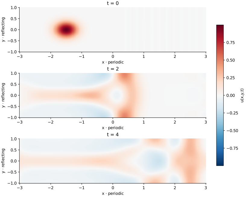
The wave tank in program 37 of Trefethen (2000) solves
\[ \begin{gathered} u_{tt}=u_{xx}+u_{yy},\\ (x,y)\in[-A,A]\times[-1,1],\\ u_y(x,\pm1,t)=0. \end{gathered} \tag{1}\]
The \(x\) direction is periodic; the top and bottom are reflecting walls. The original values are \(A=3\), \(N_x=50\) Fourier points and degree \(N_y=15\) in the Chebyshev direction. A displaced Gaussian launches a predominantly right-moving disturbance.
Let each coordinate keep its representation
For each row, the Fourier multiplier is \(-(\pi k/A)^2\). For each column, differentiate the polynomial on \(y_j=\cos(j\pi/N_y)\).
const auto laplacian = [&](const auto &values) {
  wave::Vector result(values.size());
  for (int j = 0; j <= ny; ++j) {
    for (int i = 0; i < nx; ++i) row[i] = values[index(i, j)];
    fourier.forward(row, modes);
    for (int k = 0; k <= nx / 2; ++k)
      modes[k] *= -std::pow(std::numbers::pi * k / half_length, 2);
    fourier.backward(modes, curvature);
    for (int i = 0; i < nx; ++i) result[index(i, j)] = curvature[i];
  }
  for (int i = 0; i < nx; ++i) {
    for (int j = 0; j <= ny; ++j) column[j] = values[index(i, j)];
    const auto dyy = chebyshev.derivative(column, 2);
    for (int j = 0; j <= ny; ++j) result[index(i, j)] += dyy[j];
  }
  return result;
};
The original program builds two dense differentiation matrices. Here both actions use native LocalFFT plans and the example-owned cosine map. They differentiate the same Fourier and polynomial interpolants, up to floating-point arithmetic. No public curvilinear-grid or distributed mixed-transform API is being assumed.
Solve two endpoint equations
Let \(D\) be the first derivative in \(y\), \(I\) the interior nodes and \(B=\{0,N_y\}\) the two endpoints. The wall equations are
\[ D_{BB}u_B=-D_{BI}u_I. \tag{2}\]
The endpoint rows of \(D\) are obtained by differentiating basis sample vectors once during setup. A two-by-two solve then reconstructs both boundary values after every step:
const double determinant = top[0] * bottom[ny] - top[ny] * bottom[0];
const auto enforce_neumann = [&](auto &values) {
  for (int i = 0; i < nx; ++i) {
    double rtop = 0, rbottom = 0;
    for (int j = 1; j < ny; ++j) {
      rtop -= top[j] * values[index(i, j)];
      rbottom -= bottom[j] * values[index(i, j)];
    }
    values[index(i, 0)] = (rtop * bottom[ny] - top[ny] * rbottom) / determinant;
    values[index(i, ny)] = (top[0] * rbottom - bottom[0] * rtop) / determinant;
  }
};
This imposes zero derivative, not zero value. Setting the endpoints themselves to zero would change the wall’s reflection behaviour.
for (int step = 1; step <= clock.frames * clock.gap; ++step) {
  const auto acceleration = laplacian(u);
  for (std::size_t k = 0; k < u.size(); ++k)
    next[k] = 2 * u[k] - previous[k] + clock.dt * clock.dt * acceleration[k];
  previous.swap(u);
  u.swap(next);
  enforce_neumann(u);
  if (step % clock.gap == 0) observe(step);
}
Read the first two levels carefully
The original initial field is \(\exp[-8((x+1.5)^2+y^2)]\) and its previous level shifts \(x\) by the nominal timestep \(5/(N_x+N_y^2)\). The output scheduler subsequently adjusts the step to \(2/110\). The book startup preserves this order and reconstructs the wall values after the first update, just as the original does. Its Gaussian initial level is not already an exact Neumann interpolant.
The taylor startup first reconstructs the initial boundary, then uses the adjusted step in a second-order previous level. With initial: "mode", its initial velocity is zero and the exact continuum solution is
\[ \begin{gathered} u=\cos(\pi x/A)\cos(\pi y)\cos(\omega t), \\ \omega^2=(\pi/A)^2+\pi^2. \end{gathered} \tag{3}\]
This mode checks the physical Fourier scale, both spatial derivatives, the wall equations and the time integrator together. The regression checks also compare every sample of the original Gaussian experiment with independently assembled dense derivative matrices on a small grid.
Run and experiment
openpfc run model.cpp input.json --source-root .. --launcher=noneresults/wave.csv records all nodes at each saved time. Change nx, ny or half_length, then predict which direction restricts the step. The example bounds the magnitude of the reduced Neumann operator by its maximum absolute row sum, adds the largest Fourier squared frequency, and requires \(\Delta t^2\,\mathrm{bound}<4\). For a real negative spatial eigenvalue \(-\lambda\), leapfrog needs \(\Delta t\sqrt\lambda<2\). It is a serial teaching implementation.
Download the source, input and theme helper. For a nonlinear periodic wave, continue with KdV.