OpenPFC / Waves and boundaries
A pulse meets the end of an interval
The FFT can differentiate a polynomial on a finite interval. The trick is to change the coordinate, not the boundary condition.
Download runnable lesson (.zip)
Includes the model, inputs, required headers and a short run guide.
Consider the wave equation
\[ \begin{gathered} u_{tt}=u_{xx}, \\ -1<x<1. \end{gathered} \tag{1}\]
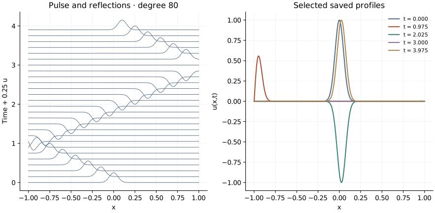
Program 19 of Trefethen (2000) starts with the narrow pulse \(u(x,0)=\exp(-200x^2)\) on \(x_j=\cos(j\pi/N)\), with \(N=80\). The pulse initially travels left, meets a fixed endpoint and reflects. This is a finite-interval problem even though its derivatives use an FFT.
Turn a polynomial into a cosine series
Write \(x=\cos\theta\). The degree-\(N\) interpolant becomes \(p(\cos\theta)=\sum_{k=0}^N a_k\cos(k\theta)\). An even extension of the samples has length \(2N\), so OpenPFC’s LocalFFT can find these coefficients. For interior points,
\[ p''(x)=\frac{p_{\theta\theta}}{\sin^2\theta} -\frac{\cos\theta\,p_\theta}{\sin^3\theta}. \tag{2}\]
Vector derivative(const Vector &u, int order) {
  if (u.size() != x.size() || (order != 1 && order != 2))
    throw std::invalid_argument("Use n+1 samples and derivative order 1 or 2");
  for (int j = 0; j < 2 * n_; ++j) extended_[j] = u[j <= n_ ? j : 2 * n_ - j];
  fft_.forward(extended_, coefficients_);
  for (int k = 0; k <= n_; ++k) {
    first_[k] = k == n_ ? 0.0 : std::complex<double>(0, k) * coefficients_[k];
    second_[k] = -static_cast<double>(k * k) * coefficients_[k];
  }
  fft_.backward(first_, theta_first_);
  if (order == 2) fft_.backward(second_, theta_second_);
  Vector result(n_ + 1);
  for (int j = 1; j < n_; ++j) {
    const double sine = std::sin(std::numbers::pi * j / n_);
    result[j] = order == 1 ? -theta_first_[j] / sine
                           : theta_second_[j] / (sine * sine) -
                                 x[j] * theta_first_[j] / (sine * sine * sine);
  }
  // Analytic limits of T'_k and T''_k avoid dividing by sin(theta)=0.
  for (int k = 1; k <= n_; ++k) {
    const double a = coefficients_[k].real() / (k == n_ ? 2 * n_ : n_);
    const double endpoint = order == 1 ? k * k : k * k * (k * k - 1.0) / 3;
    result[0] += a * endpoint;
    result[n_] += a * endpoint * ((k + order) % 2 ? -1 : 1);
  }
  return result;
}
The odd derivative sets the Nyquist multiplier to zero. The second derivative retains it. At the two endpoints the helper uses the exact polynomial limits \(T'_k(1)=k^2\) and \(T''_k(1)=k^2(k^2-1)/3\), with the appropriate signs at \(-1\). Dividing by a tiny sine there would magnify roundoff.
The book calls chebfft twice. Applying the chain rule directly gives the same second derivative of the interpolating polynomial, using one forward and two inverse transforms. This example-owned mapping is not a public OpenPFC nonuniform-grid operator.
Remember two time levels
Leapfrog for Equation 1 uses
\[ u^{m+1}=2u^m-u^{m-1}+\Delta t^2D_{xx}u^m. \tag{3}\]
for (int step = 1; step <= clock.frames * clock.gap; ++step) {
  auto acceleration = derivative.derivative(u, 2);
  acceleration.at(0) = acceleration.at(n) = 0;
  for (int j = 0; j <= n; ++j)
    next[j] = 2 * u[j] - previous[j] + clock.dt * clock.dt * acceleration[j];
  previous.swap(u);
  u.swap(next);
  if (step % clock.gap == 0) observe(step);
}
Endpoint acceleration is zero, as in the original program. The supplied two endpoint levels therefore determine a linear-in-time endpoint value. For this Gaussian their magnitudes are about \(10^{-87}\); this is an excellent approximation to fixed zero ends, but it is useful to say what the recurrence actually imposes.
The previous level is an initial condition
The default startup: "book" uses the original \(u^{-1}_j=\exp[-200(x_j-\Delta t_{\rm nominal})^2]\). It approximates initial velocity \(u_t(x,0)=u_x(x,0)\). The output interval is .075; rounding the number of steps gives \(\Delta t=.00125\). Rounding the number of frames makes the actual final time 3.975, rather than 4. Every CSV row records its actual time.
Set startup: "taylor" to use \(u^{-1}=u^0-\Delta t\,u_t^0+\tfrac12\Delta t^2D_{xx}u^0\). This uses the adjusted timestep consistently. Set initial: "mode" as well to start with \(\cos(\pi x/2)\) and zero velocity. Then compare with the exact solution \(\cos(\pi x/2)\cos(\pi t/2)\). At a resolved spatial degree, halving the Taylor-started timestep should reduce the temporal error by about four.
Run and change it
openpfc run model.cpp input.json --source-root .. --launcher=noneresults/wave.csv contains all nodes at every saved level. Try changing n, then predict why an endpoint-clustered grid needs \(\Delta t=O(N^{-2})\) for an explicit wave equation. The program bounds the adjusted step by dt*n*n <= 8. This complete-domain reference runs on one process.
Keep the C++ model, input and theme helper together. Continue with a square wave problem.