OpenPFC / Nonlinear waves

Let dispersion evolve exactly between stages

A stiff linear oscillation has a known solution. Factor it out and let Runge–Kutta handle the nonlinear part.

Includes the model, inputs, required headers and a short run guide.

The Korteweg–de Vries equation combines nonlinear steepening with dispersion:

\[ \begin{gathered} u_t+u\,u_x+u_{xxx}=0, \\ -\pi\le x<\pi. \end{gathered} \tag{1}\]

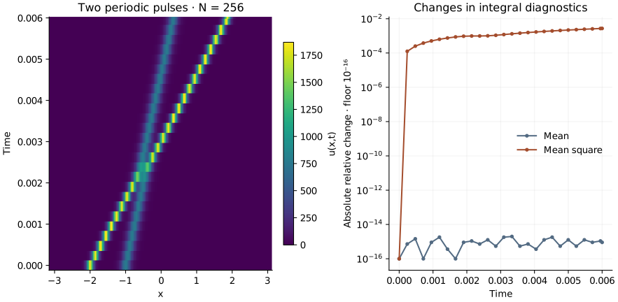
Program 27 of Trefethen (2000) starts two narrow solitary-wave profiles with amplitudes \(3A^2\) and \(3B^2\), where \(A=25\) and \(B=16\). Their centres are initially \(-2\) and \(-1\). The larger pulse moves faster, catches the smaller one and emerges from the interaction. The finite periodic domain and sampled initial data define a numerical experiment; an isolated infinite-line soliton is not an exact answer to this two-pulse periodic initial-value problem.

Separate the Fourier equation

Using \(\widehat{\partial_xu}_k=ik\hat u_k\) gives

\[ \frac{d\hat u_k}{dt}=ik^3\hat u_k-\frac{ik}{2}\widehat{u^2}_k. \tag{2}\]

Set \(L_k=ik^3\) and \(v_k(t)=e^{-tL_k}\hat u_k(t)\). Then

\[ \begin{aligned} v'_k&=e^{-tL_k}\mathcal N_k(e^{tL}v),\\ \mathcal N_k(\hat u)&=-\frac{ik}{2} \mathcal F\{[\mathcal F^{-1}\hat u]^2\}_k. \end{aligned} \tag{3}\]

This is an ordinary, time-dependent ODE for complex coefficients. OpenPFC’s ExplicitRKStepper accepts a complex scalar state and a real RK4 tableau:

for (int k = 0; k <= n / 2; ++k)
  linear[k] = std::complex<double>(0, k == n / 2 ? 0 : k * k * k);
const auto rhs = [&](double t, const auto &v, auto &dv) {
  for (int k = 0; k <= n / 2; ++k)
    physical_modes[k] = std::exp(t * linear[k]) * v[k];
  fft.backward(physical_modes, u);
  for (int j = 0; j < n; ++j) square[j] = u[j] * u[j];
  fft.forward(square, nonlinear);
  for (int k = 0; k <= n / 2; ++k) {
    const double odd_k = k == n / 2 ? 0 : k;
    dv[k] = std::exp(-t * linear[k]) *
            std::complex<double>(0, -.5 * nonlinearity * odd_k) * nonlinear[k];
  }
};
pfc::sim::steppers::ExplicitRKStepper<decltype(rhs), std::complex<double>>
    stepper(dt, transformed.size(),
            pfc::sim::steppers::make_rk4_classical<double>(), rhs);

LocalFFT has an unscaled forward transform and a normalized inverse. No extra factor of \(N\) belongs in the product. Its half-spectrum stores the Hermitian coefficients of a real field. Both odd multipliers use zero at the Nyquist mode, matching the original program.

The book writes its integrating-factor RK4 stages explicitly, resetting the factor each step. Here the public RK4 stepper integrates the global transformed variable. These are algebraically equivalent updates, with different floating-point roundoff. An independent reference checks the original full-complex-FFT stage formula.

for (int step = 1; step <= steps; ++step) {
  stepper.step((step - 1) * dt, transformed);
  if (step % gap == 0 || step == steps) observe(step);
}

Figure 1: Native snapshots of the two-pulse interaction, followed by relative changes in the mean and mean-square diagnostics. Changes below 10⁻¹⁶ are placed at that floor for the logarithmic display.

Preserve the distinction between a method and an invariant

The zero nonlinear multiplier preserves the mean coefficient. The continuum equation also conserves \(\int u^2\,dx\). A finite timestep and an aliased pointwise product need not preserve that second quantity exactly. The diagnostic CSV records both; it does not enforce them. The displayed \(N=256\) run changes the mean square by a few parts per thousand. This is a reason to compare grid and timestep refinements, even though the mean remains at roundoff accuracy.

The original experiment uses \(N=256\), \(\Delta t=.4/N^2\) and final time .006. It does not de-alias the product. This reproduction keeps that choice visible. Adding padding or a mode filter changes the discrete method and should be compared explicitly.

Try a problem with a known answer

Set initial: "cosine" and nonlinearity: 0. Dispersion alone then gives \(u(x,t)=\cos(2x+8t)\). The transformed state is constant, so RK4 adds no time-discretization error to this linear check. With initial: "constant", both derivatives vanish and the full nonlinear problem should preserve the constant field.

For the nonlinear interaction, halve dt while keeping the same grid and compare the whole final field. Refining only the step cannot remove spatial truncation or aliasing errors.

openpfc run model.cpp input.json --source-root .. --launcher=none

The complete-domain example runs on one process. It saves all physical nodes in results/kdv.csv and integral diagnostics in results/diagnostics.csv. The last step is always saved, even when it does not coincide with save_every. Step counts round end/dt, and every output includes its actual time.

Keep the model, input and shared I/O helper together. Compare the integrating factor with ETD step doubling: both use linear exponentials, but their nonlinear stage formulas differ.

References

Trefethen, Lloyd N. 2000. Spectral Methods in MATLAB. Society for Industrial; Applied Mathematics. https://doi.org/10.1137/1.9780898719598.