OpenPFC / Waves and boundaries
Let a wave spread across a square
A two-dimensional Laplacian is the sum of two one-dimensional operations. Keep that structure visible in the code.
Download runnable lesson (.zip)
Includes the model, inputs, required headers and a short run guide.
A pulse spreads and reflects in \([-1,1]^2\):
\[ \begin{aligned} u_{tt}&=u_{xx}+u_{yy},\\ u(x,y,0)&=\exp\{-40[(x-.4)^2+y^2]\}. \end{aligned} \tag{1}\]
Program 20 of Trefethen (2000) uses degree 24 in each coordinate and leapfrog in time. Both spatial coordinates are Chebyshev coordinates. Its title says “via FFT” because cosine-mapped differentiation uses transforms; the physical square is not periodic.
Reuse a line derivative in two directions
The one-dimensional lesson derives the even extension and the chain rule. Here the same helper acts on every interior row and column:
const auto laplacian = [&](const auto &values) {
  wave::Vector result(values.size());
  for (int j = 1; j < n; ++j) {
    for (int i = 0; i <= n; ++i) line[i] = values.at(index(i, j));
    const auto dxx = derivative.derivative(line, 2);
    for (int i = 1; i < n; ++i) result[index(i, j)] = dxx.at(i);
  }
  for (int i = 1; i < n; ++i) {
    for (int j = 0; j <= n; ++j) line[j] = values.at(index(i, j));
    const auto dyy = derivative.derivative(line, 2);
    for (int j = 1; j < n; ++j) result[index(i, j)] += dyy.at(j);
  }
  return result;
};
Only interior acceleration is filled. The full state still contains the boundary samples needed by the interpolating polynomial. With \(u^{-1}=u^0\), zero boundary acceleration preserves their initial values. Those Gaussian tails are small, but not exactly zero: the largest is about \(5.6\times10^{-7}\). We retain them to reproduce the original discrete problem.
This tensor application costs \(O(N^2\log N)\) and stores \(O(N^2)\) field values. It avoids constructing a square two-dimensional derivative matrix. The helper creates its FFT plan once and reuses it for every line.
Advance the field after calculating its whole acceleration
for (int step = 1; step <= clock.frames * clock.gap; ++step) {
  const auto acceleration = laplacian(u);
  for (std::size_t j = 0; j < u.size(); ++j)
    next[j] = 2 * u[j] - previous[j] + clock.dt * clock.dt * acceleration[j];
  previous.swap(u);
  u.swap(next);
  if (step % clock.gap == 0) observe(step);
}
Two swaps rotate the three buffers. Every derivative sees the complete old field; an in-place cell-by-cell update would change the method. The original \(\Delta t=6/N^2\) divides the output interval \(1/3\) into 32 steps, giving \(\Delta t=1/96\) and snapshots at 0, 1/3, 2/3 and 1.
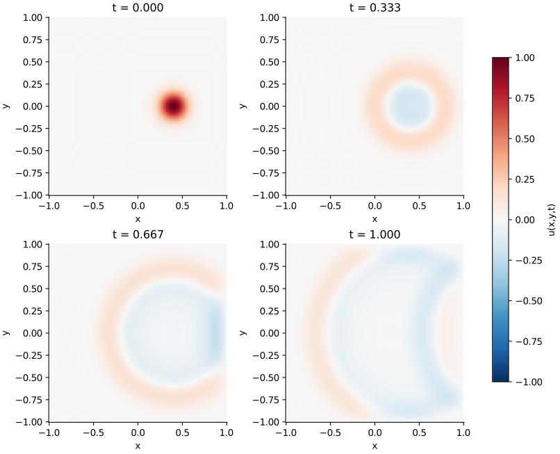
The book uses cubic interpolation for its display. This figure evaluates the saved degree-24 polynomial barycentrically in both directions. The fine display grid does not increase the simulation’s resolution.
Ask what zero velocity means numerically
The default startup: "book" sets \(u^{-1}=u^0\). In the first update this gives \(u^1=u^0+\Delta t^2\Delta_hu^0\). A Taylor expansion for zero initial velocity has half that acceleration term. Consequently the book startup introduces a first-order initial-velocity error.
Use startup: "taylor" for \(u^{-1}=u^0+\tfrac12\Delta t^2\Delta_hu^0\). With initial: "mode", the continuum answer is
\[ u(x,y,t)=\cos(\pi x/2)\cos(\pi y/2) \cos(\pi t/\sqrt2). \tag{2}\]
Compare both startups at two timesteps. The spatial operator and leapfrog recurrence stay the same; the initial level explains the different convergence rates.
Run and inspect
openpfc run model.cpp input.json --source-root .. --launcher=noneresults/wave.csv contains all \((N+1)^2\) samples per saved time. The model checks dt*n*n <= 6 after output-time adjustment and runs on one process. Keep the source, input and shared FFT helper together. Next combine periodic and reflecting directions.