OpenPFC / How stable is a spectrum?
Eigenvalue dots do not tell the whole story
An eigenvalue is one point. A small perturbation can make a whole region relevant.
Download runnable lesson (.zip)
Includes the model, inputs, required headers and a short run guide.
The real harmonic oscillator has a familiar spectrum. Program 24 of Trefethen (2000) changes the potential to a complex one on the interval \((-6,6)\):
\[ \begin{aligned} Au&=-u''+(1+3i)x^2u,\\ u(-6)&=u(6)=0. \end{aligned} \tag{1}\]
The resulting matrix is nonnormal. Its eigenvalues alone do not describe how it responds to perturbations. This chapter reproduces the book’s degree-70 grid, all 69 finite-matrix eigenvalues, and the 546 points of its complex-plane sampling grid.
Build the operator with native derivatives
Map the Lobatto coordinate \(\xi\in[-1,1]\) to \(x=L\xi\), with \(L=6\). The second derivative acquires a factor \(1/L^2\). Apply native OpenPFC Chebyshev differentiation twice to each interior nodal basis function:
for (int j = 1; j < n; ++j) {
  polynomial::Vector unit(n + 1);
  unit[j] = 1;
  const auto first = pfc::fft::chebyshev_derivative(unit);
  const auto second = pfc::fft::chebyshev_derivative(first);
  for (int i = 1; i < n; ++i) a[i - 1][j - 1] = -second[i] / (length * length);
  a[j - 1][j - 1] += Complex(1, 3) * std::pow(length * x[j], 2);
}
const auto modes = eigen_reference::solve(a);
The first derivative includes both endpoint values before taking the second derivative. Restrict the resulting second derivative to interior equations afterwards. Squaring an already restricted first derivative would produce a different operator.
The eigenvalues are those of this finite interval and collocation matrix. The infinite-line values \((2j+1)\sqrt{1+3i}\) provide a check for the first few modes, rather than an exact reference for every high discrete mode.
Ask how close a shifted matrix is to singular
At an eigenvalue, \(zI-A\) is singular. Away from the eigenvalues, the smallest singular value measures the smallest matrix perturbation that would make it singular:
\[ \begin{aligned} \Lambda_\varepsilon(A) &=\{z:\sigma_{\min}(zI-A)\le\varepsilon\}\\ &=\bigcup_{\|E\|_2\le\varepsilon}\operatorname{spec}(A+E). \end{aligned} \tag{2}\]
For an invertible shift, this is also the reciprocal of the resolvent norm: \(\|(zI-A)^{-1}\|_2=1/\sigma_{\min}(zI-A)\). The experiment uses the ordinary Euclidean norm of the nodal vectors, as in the book. A weighted energy norm or a different basis would define a different perturbation question.
for (int iy = 0; iy <= static_cast<int>(40 / step); ++iy)
  for (int ix = 0; ix <= static_cast<int>(50 / step); ++ix) {
    const Complex z(ix * step, iy * step);
    auto shifted = a;
    for (auto &row : shifted)
      for (auto &value : row) value = -value;
    for (int j = 0; j < n - 1; ++j) shifted[j][j] += z;
    output << z.real() << ',' << z.imag() << ','
           << singular_values::smallest(shifted) << '\n';
  }
Keep the small singular values
The example-owned reference uses one-sided complex Jacobi rotations. For each pair of columns, compute their norms and inner product, then apply a unitary rotation that reduces their overlap. Once all pairs are orthogonal to floating-point tolerance, the column norms are the singular values. The source helper also scales the input and imposes an iteration limit.
for (int sweep = 0; sweep < 100; ++sweep) {
  bool rotated = false;
  for (int p = 0; p < n; ++p)
    for (int q = p + 1; q < n; ++q) {
      double alpha = 0, beta = 0;
      Complex gamma = 0;
      for (int i = 0; i < n; ++i) {
        alpha += std::norm(columns[p][i]);
        beta += std::norm(columns[q][i]);
        gamma += std::conj(columns[p][i]) * columns[q][i];
      }
      const double overlap = std::abs(gamma);
      if (overlap <= tolerance * std::sqrt(alpha) * std::sqrt(beta)) continue;
      const double tau = (beta - alpha) / (2 * overlap);
      const double t =
          std::copysign(1.0, tau) / (std::abs(tau) + std::hypot(1.0, tau));
      const double c = 1 / std::sqrt(1 + t * t);
      const Complex s = c * t * gamma / overlap;
      for (int i = 0; i < n; ++i) {
        const Complex left = columns[p][i], right = columns[q][i];
        columns[p][i] = c * left - std::conj(s) * right;
        columns[q][i] = s * left + c * right;
      }
      rotated = true;
    }
  if (!rotated) {
    double minimum = std::numeric_limits<double>::infinity();
    for (const auto &column : columns) {
      double norm2 = 0;
      for (auto value : column) norm2 += std::norm(value);
      minimum = std::min(minimum, std::sqrt(norm2));
    }
    return scale * minimum;
  }
}
Forming \((zI-A)^*(zI-A)\) would square the condition number. Its smallest eigenvalue can lose the very information the plot is meant to show. The column-rotation calculation works on the shifted matrix itself. For the relative-accuracy analysis of one-sided Jacobi, see Demmel and Veselić (1992). It remains a bounded educational implementation, with input roundoff and convergence limits; it is not a rank certificate or a new public OpenPFC SVD API.
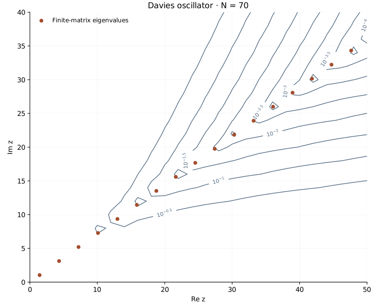
Contour lines interpolate the samples. A small region around an eigenvalue can fall between sample points and remain undrawn; refining step tests this drawing resolution.
Reproduce the picture, then change the question
openpfc run model.cpp input.json --source-root .. --launcher=noneThe default input uses \(N=70\), \(L=6\) and increments of two on \(\operatorname{Re}z=0,2,\ldots,50\) and \(\operatorname{Im}z=0,2,\ldots,40\), matching the original program. results/spectrum.csv stores all eigenvalues and their residuals; results/pseudospectrum.csv stores every sampled singular value.
Reduce step to 1 and then 0.5 to refine the contour drawing. That adds shifted singular-value calculations; it does not improve the spatial operator. Change n separately to test collocation resolution, and change length separately to test the finite-interval truncation. Predict which change should move eigenvalue dots and which should only make a contour smoother. The denser plane sampling is substantially slower.
The ordinary numerical checks compare complete coarse complex-plane grids at degrees 12 and 70 with inverse iteration through independently assembled shifted solves. The even and odd reflection sectors separate nearly equal singular-value pairs before that inverse iteration. This avoids both the C++ Jacobi algorithm and explicit normal equations. The native helper checks include complex triangular matrices with singular values as small as \(10^{-12}\). Separate qualification compares every value of the original 546-point degree-70 plot with SciPy’s SVD. SciPy is not a runtime or routine-test dependency.
This complete-domain reference runs on one process and accepts degrees 6 through 80, half-lengths 2 through 12, and complex-plane increments 0.5 through 10. Keep the source, singular-value helper, eigensolver and collocation helper together. Continue to the Orr–Sommerfeld example to see why sensitivity and resolution matter for a small growth rate.