OpenPFC / Growth rates need a resolution check
A tiny real part decides whether a disturbance grows
A complex eigenvalue gives a frequency and a growth rate. Near neutral stability, the small part of the answer matters most.
Download runnable lesson (.zip)
Includes the model, inputs, required headers and a short run guide.
Program 40 of Trefethen (2000) studies a small disturbance to flow between parallel walls. The base velocity is \(U(y)=1-y^2\), with walls at \(y=\pm1\). Scale velocity by the centreline speed and length by the channel half-height; their product divided by kinematic viscosity is the Reynolds number \(R\).
Seek a wall-normal velocity disturbance proportional to \(v(y)e^{\lambda t+ix}\). This fixes the streamwise wave number to one. The Orr–Sommerfeld equation becomes
\[ \begin{aligned} \lambda(D^2-1)v &=\frac{D^4-2D^2+1}{R}v\\ &\quad-iU(D^2-1)v-2iv,\\ v(\pm1)&=v'(\pm1)=0, \end{aligned} \tag{1}\]
where \(D=d/dy\). The real part of \(\lambda\) determines exponential growth or decay. The imaginary part determines the oscillation; with this wave convention the phase speed is \(-\operatorname{Im}\lambda\).
Reuse the clamped fourth derivative
The beam and plate chapters already built the two required operators from native OpenPFC Chebyshev differentiation. Reuse the weighted, clamped \(D_4\) and the ordinary interior \(D_2\) from the book. The generalized matrix problem is
\[ \begin{gathered} Av=\lambda Bv, \\ B=D_2-I, \end{gathered} \tag{2}\]
\[ \begin{aligned} A&=\frac{D_4-2D_2+I}{R}-2iI\\ &\quad-i\operatorname{diag}(U)B. \end{aligned} \tag{3}\]
Multiplication by \(U\) acts on each row of \(B\). Moving it to the other side would change the operator: differentiation and multiplication do not commute.
for (int i = 0; i < m; ++i)
  for (int j = 0; j < m; ++j) {
    const double identity = i == j ? 1 : 0;
    const double base_velocity = 1 - op.x[i + 1] * op.x[i + 1];
    b[i][j] = op.laplacian[i][j] - identity;
    a[i][j] =
        (op.biharmonic[i][j] - 2 * op.laplacian[i][j] + identity) / reynolds -
        imaginary * (2 * identity + base_velocity * b[i][j]);
  }
Solve a mass system before the ordinary eigenproblem
For these Dirichlet interior values, \(B=D_2-I\) is invertible. Solve the multiple-right-hand-side system \(BC=A\), then find \(Cv=\lambda v\):
const auto evolution = pencil::mass_solve(b, a);
const auto modes = eigen_reference::solve(evolution);
const auto leading = modes.back().value;
The example-owned helper uses elimination with partial pivoting for the real mass matrix and complex right-hand sides. It solves for \(C\) directly; it does not construct a separate inverse of \(B\). The existing bounded complex shifted-QR reference handles the resulting dense eigenproblem. This is an educational reduction of this invertible pencil, rather than a public OpenPFC generalized eigensolver. A general pencil can have a singular \(B\) and needs a method such as QZ instead.
The separate qualification compares every eigenvalue at all four original resolutions with SciPy’s generalized eigensolver, using independently differentiated Lagrange products for the operators. SciPy is a qualification tool, not a dependency of the C++ model or the ordinary example tests. That QZ calculation scales each row of both \(A\) and \(B\) by the same positive factor, the reciprocal of the largest absolute entry in that row of \(A\). Premultiplication by this invertible diagonal matrix preserves the generalized eigenvalues and reduces the range of row magnitudes. At degree 100, the unscaled calculation loses accuracy in the leading root; equilibration brings it into agreement with the other checks.
Look at all four resolutions
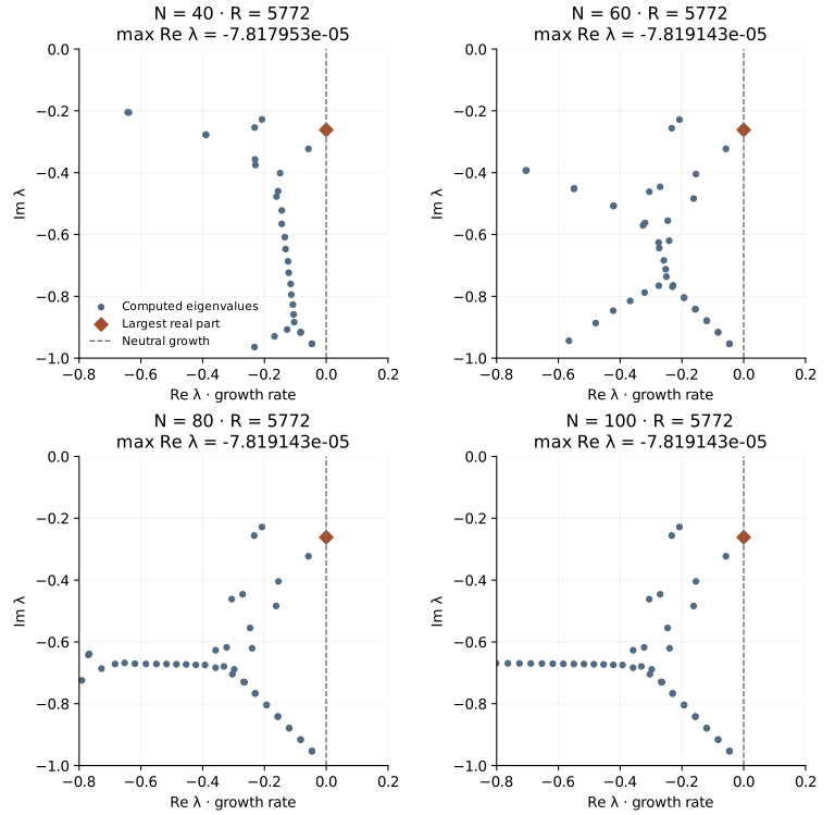
openpfc run model.cpp input.json --source-root .. --launcher=noneThe default input uses \(R=5772\) and degrees 40, 60, 80 and 100, matching the original program. results/spectrum.csv contains every eigenvalue and both residuals; results/vectors.csv contains every complex nodal eigenvector, including the zero endpoint values. results/growth.csv records the eigenvalue with the largest real part at each resolution. The default leading growth rate is approximately \(-7.81914\times10^{-5}\) at the three finest degrees. It is negative for this fixed wave number; the apparent proximity to the neutral line in the plot needs the numerical resolution comparison, rather than a visual guess.
Separate three different checks
The transformed residual checks \(Cv-\lambda v\). The model also computes the original-pencil residual
\[ \eta=\frac{\|Av-\lambda Bv\|_2} {(\|A\|_F+|\lambda|\|B\|_F)\|v\|_2}. \tag{4}\]
This is a scaled backward-residual check, not an error bound for an eigenvalue. The operator is nonnormal: its eigenvectors need not be orthogonal, and small perturbations need not produce proportionally small eigenvalue changes. Compare resolutions before trusting the sign of a small growth rate.
The ordinary numerical test independently differentiates Lagrange products, checks every generalized eigenvector, verifies the full spectrum’s trace and uses generalized inverse iteration to check the leading mode. It also runs the higher-Reynolds-number input:
openpfc run model.cpp unstable.json --source-root .. --launcher=noneFirst predict how reducing viscosity changes the competition between diffusion and shear. Then compare the leading growth rates at \(R=5772\) and \(R=10000\), and repeat with another resolution. The fixed wave number means this experiment does not search the critical Reynolds number over all possible wavelengths. It is a linear disturbance calculation, not a nonlinear channel-flow simulation.
This complete-domain reference runs on one process. Keep the source, pencil helper, clamped helper, eigensolver and collocation helper together. Inputs accept one through eight even degrees between 12 and 100 and Reynolds numbers between 100 and one million.