OpenPFC / Operators and their solutions
Find the energies of a harmonic trap
Build a Fourier Hamiltonian with the native local FFT and watch its lowest energies converge to odd integers.
Download runnable lesson (.zip)
Includes the model, inputs, required headers and a short run guide.
An eigenvalue problem asks which shapes an operator preserves up to a scalar. Program 8 of Trefethen (2000) considers the harmonic oscillator
\[-u''+x^2u=\lambda u,\qquad x\in\mathbb R.\]
Its exact square-integrable energies are \(1,3,5,7,\ldots\). We repeat the book’s periodic truncation to \([-8,8]\) and its resolutions 6,12,…,36. There are two approximations to distinguish: truncating the infinite line and resolving the resulting finite interval.
Assemble an operator by applying it to basis vectors
The native local FFT transforms one coordinate basis vector at a time. Multiplying its Fourier coefficients by \(k^2\) applies \(-\partial_{xx}\); the normalized inverse gives one matrix column. This deliberately small \(O(N^2\log N)\) construction makes the operator explicit for an example-owned symmetric eigensolver. A large calculation would apply it without assembling all the columns.
inline Matrix negative_laplacian(int n, double length) {
  pfc::fft::LocalFFT fft({n, 1, 1});
  Matrix a(n, Vector(n));
  for (int column = 0; column < n; ++column) {
    Vector basis(n), image(n);
    basis[column] = 1;
    pfc::fft::ComplexVector coefficients(n / 2 + 1);
    fft.forward(basis, coefficients);
    for (int k = 0; k <= n / 2; ++k) {
      const double wave = 2 * std::numbers::pi * k / length;
      coefficients[k] *= wave * wave;
    }
    fft.backward(coefficients, image);
    for (int row = 0; row < n; ++row) a[row][column] = image[row];
  }
  return a;
}
The even-grid Nyquist second derivative is retained. Squaring a real-grid first derivative that suppresses its Nyquist mode would give a different second derivative. The physical wave number is \(2\pi k/16\), not simply \(k\).
for (int n : sizes) {
  if (n < 6 || n > 128 || n % 2)
    throw std::invalid_argument("Use even n in [6,128]");
  constexpr double length = 16;
  const double h = length / n;
  const auto domain = pfc::domain::create(pfc::GridSize{{n, 1, 1}},
                                          pfc::PhysicalOrigin{{-8 + h, 0, 0}},
                                          pfc::GridSpacing{{h, 1, 1}});
  pfc::data::Field<double> potential(domain, pfc::domain::index_box(domain), 0);
  potential.apply([](double x, double, double) { return x * x; });
  auto hamiltonian = fourier_matrix::negative_laplacian(n, length);
  for (int j = 0; j < n; ++j) hamiltonian[j][j] += potential(j, 0, 0);
  const auto energies = fourier_matrix::eigenvalues(hamiltonian);
  for (int mode = 0; mode < 4; ++mode)
    output << n << ',' << mode + 1 << ',' << energies[mode] << ','
           << 2 * mode + 1 << '\n';
}
The field supplies physical coordinates for the potential. Its first sample is \(-8+h\), matching the book’s cyclic shift of a periodic grid; \(-8\) and \(8\) are periodic images. The potential and the low-energy modes are not periodic functions on the whole real line. The finite-domain calculation is an approximation, justified for modes that are tiny near the chosen endpoints.
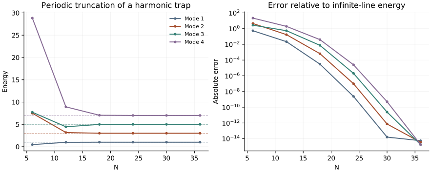
Refine one approximation at a time
openpfc run model.cpp input.json --source-root .. --launcher=noneresults/energies.csv records all four energies at each input resolution. Zero floating-point differences appear at the \(10^{-16}\) display floor of the logarithmic error plot; the CSV retains the computed energies. The native FFT and field are public OpenPFC interfaces; the small dense Jacobi diagonalization in matrix.hpp belongs to this experiment. No public eigensolver API is implied. The check compares the FFT-built operator with an independent direct DFT and verifies convergence toward the odd integers. Increasing \(N\) cannot remove an error caused by choosing an insufficiently large physical interval. Compare next with a periodic potential, whose spectrum changes for a different physical reason.
The complete C++ model and starting input are available with this lesson. Keep the shared matrix.hpp one directory above the model.