A square can sing the same note in two shapes

OpenPFC / Symmetry and vibration

A square can sing the same note in two shapes

Twenty-five shapes come from one operator. Repeated frequencies tell us something about the square.

Download runnable lesson (.zip)

Includes the model, inputs, required headers and a short run guide.

The beam lesson fixed both displacement and slope at each end. Program 39 of Trefethen (2000) asks the corresponding question on the square \((-1,1)^2\):

\[ \begin{gathered} \Delta^2 u=\lambda u, \\ u=\partial_n u=0\quad\text{on all four edges}. \end{gathered} \tag{1}\]

For a uniform thin plate, the dimensional material and length factors multiply every frequency in the same way. The dimensionless ratios \(\omega_j/\omega_1=\sqrt{\lambda_j/\lambda_1}\) therefore describe the relative notes without choosing a particular material.

Assemble a two-dimensional action from one-dimensional operators

The identity \(\Delta^2=\partial_x^4+2\partial_x^2\partial_y^2+\partial_y^4\) gives the book’s discrete operator

\[ L=I\otimes D_4+D_4\otimes I+2D_2\otimes D_2. \tag{2}\]

Here \(D_4\) is the weighted clamped operator from the beam chapter, built from native OpenPFC Chebyshev differentiation. \(D_2\) is the ordinary second-derivative matrix restricted to interior values with zero endpoint values, as in the book. The complete matrices are formed before restricting their rows and columns. Simply squaring the interior \(D_2\) would impose a different fourth-order boundary problem.

Keep \(x\) as the fastest index. Apply each factor along its own axis:

for (int j = 0; j < m; ++j)
  for (int i = 0; i < m; ++i)
    for (int k = 0; k < m; ++k) {
      result[i + m * j] +=
          op.biharmonic[i][k] * u[k + m * j] + op.biharmonic[j][k] * u[i + m * k];
      xx[i + m * j] += op.laplacian[i][k] * u[k + m * j];
    }
for (int j = 0; j < m; ++j)
  for (int i = 0; i < m; ++i)
    for (int k = 0; k < m; ++k)
      result[i + m * j] += 2 * op.laplacian[j][k] * xx[i + m * k];

This action avoids storing a full tensor matrix. The small matrices used for the eigenproblem below are projections of this same action.

Let symmetry separate the repeated modes

Reflection in either coordinate leaves the plate unchanged. Choose a basis whose vectors are even or odd under each reflection. Within the even/even and odd/odd sectors, also split into shapes that are symmetric or antisymmetric under \(x\leftrightarrow y\).

For an orthonormal nodal basis \(Q\), form \(Q^T LQ\):

for (int column = 0; column < size; ++column) {
  const auto image = plate::apply(op, basis[column]);
  for (int row = 0; row < size; ++row)
    reduced[row][column] = std::inner_product(
        basis[row].begin(), basis[row].end(), image.begin(), 0.0);
}
const auto eigenpairs =
    eigen_reference::solve(eigen_reference::complex_matrix(reduced));

The example-owned shifted-QR reference solves each small dense block. It is the same numerical eigenproblem as the book’s full matrix; the symmetry split chooses interpretable shapes inside repeated eigenspaces. An even/odd mode has an odd/even partner obtained by transposing its nodal array. Those partners have the same eigenvalue and independent shapes. Other linear combinations of a repeated pair are equally valid.

const auto op = clamped::operators(n);
const auto modes = plate::modes(op);
const double fundamental = modes.front().eigenvalue;

Draw a shape that respects the clamp

The display uses a tensor product of the beam’s weighted cardinal basis. Each one-dimensional basis function vanishes with its first derivative at both endpoints. Values and normal slopes consequently vanish along every edge of the reconstructed surface:

for (int b = 0; b < m; ++b)
  for (int a = 0; a < m; ++a) {
    const double coefficient = mode.u[a + m * b];
    u += basis.value[i][a] * basis.value[j][b] * coefficient;
    ux += basis.slope[i][a] * basis.value[j][b] * coefficient;
    uy += basis.value[i][a] * basis.slope[j][b] * coefficient;
  }

This display uses the constrained polynomial rather than the book’s cubic image interpolation. The mixed derivative in the collocation operator still uses the book’s ordinary \(D_2\); it is not redefined by the display interpolation.

Figure 1: The first 25 clamped-plate modes at degree 17. Blue and red distinguish the two signs of each normalized shape; black curves mark zero displacement. Each panel gives the mode number and its frequency relative to the fundamental. The sign and orientation of a mode are arbitrary.

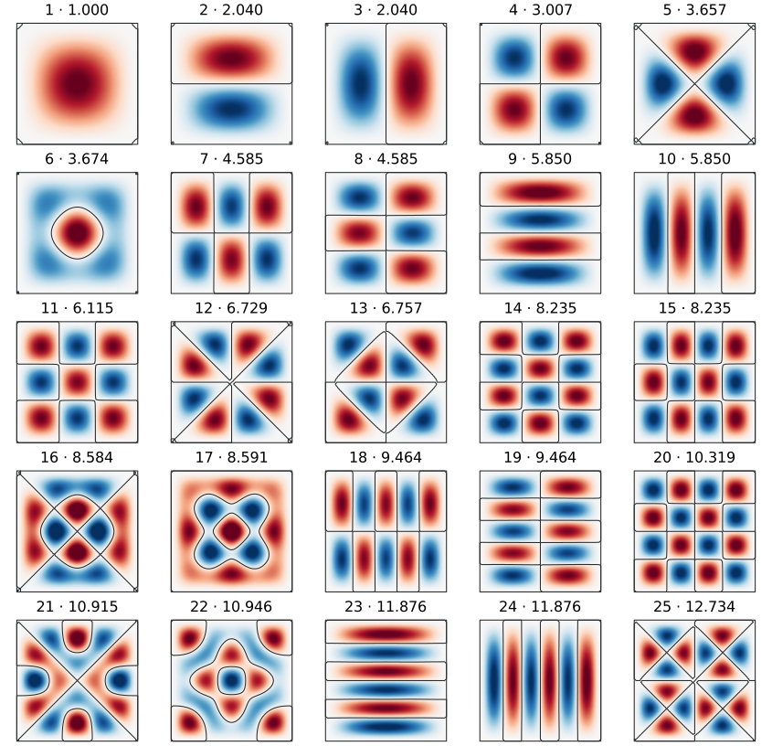
Open the full-size mode gallery to inspect individual nodal lines on a small screen.

Check the operator, the edges and the eigenspace

The model records all 25 eigenvalues, relative frequencies, symmetry labels and complete nodal and display fields. It checks the full operator residual after lifting each reduced eigenvector. The numerical regression differentiates Lagrange products independently, checks those residuals, verifies the clamped edges and checks that equal-frequency partners are independent.

openpfc run model.cpp input.json --source-root .. --launcher=none

Try degree 10 and then 17. Compare the low frequencies before inspecting the more demanding high modes. Against degree 20, the fundamental eigenvalue changes by about \(6\times10^{-7}\) at degree 10, but the largest relative change among the first 25 eigenvalues is about \(0.29\). At degree 17 those differences fall to about \(1.5\times10^{-9}\) and \(5.3\times10^{-6}\). These are comparisons between resolutions, rather than errors against an exact continuum spectrum. Refinement tests convergence of the collocation approximation; a small matrix residual alone does not show that a continuum mode is resolved. This complete-domain teaching reference runs on one process and accepts degrees 6 through 20.

Keep the source, input, plate helper, clamped helper, eigensolver and collocation helper together.

References

Trefethen, Lloyd N. 2000. Spectral Methods in MATLAB. Society for Industrial; Applied Mathematics. https://doi.org/10.1137/1.9780898719598.