OpenPFC / Four derivatives, four endpoint conditions
Build the clamped ends into the trial function
A zero value and a zero slope are different conditions. Choose a representation that satisfies both.
Download runnable lesson (.zip)
Includes the model, inputs, required headers and a short run guide.
Program 38 of Trefethen (2000) solves a dimensionless clamped beam problem:
\[ \begin{aligned} u^{(4)}(x)&=e^x,\qquad -1<x<1,\\ u(\pm1)&=u'(\pm1)=0. \end{aligned} \tag{1}\]
The degree-15 grid is small enough to expose the whole construction. Deleting the endpoint rows of an ordinary fourth-derivative matrix would impose only two of the required conditions.
Use the native Chebyshev building blocks
OpenPFC provides Lobatto nodes and a complete-domain FFT-based first derivative. Apply that derivative to the nodal basis vectors to obtain the matrix representation:
const auto x = pfc::fft::chebyshev_lobatto(n);
polynomial::Matrix d(n + 1, polynomial::Vector(n + 1));
polynomial::Vector basis(n + 1);
for (int j = 0; j <= n; ++j) {
  basis.at(j) = 1;
  const auto column = pfc::fft::chebyshev_derivative(basis);
  for (int i = 0; i <= n; ++i) d[i][j] = column[i];
  basis[j] = 0;
}
The earlier differentiation lesson develops reference formulas so you can see the polynomial mathematics. Here the native chebyshev_derivative supplies the same operation directly. The example-owned helper composes it into a constrained fourth derivative; it does not add a new public beam solver.
Put both endpoint conditions in the representation
Write \(u(x)=(1-x^2)v(x)\), where the degree-\(N\) polynomial \(v\) has \(v(\pm1)=0\). Then both \(u\) and \(u'=-2xv+(1-x^2)v'\) vanish at the ends. Differentiating four times gives
\[ u^{(4)}=(1-x^2)v^{(4)}-8xv^{(3)}-12v''. \tag{2}\]
At interior nodes, \(v_j=u_j/(1-x_j^2)\). That identity gives the weighted matrix from the book:
for (int i = 1; i < n; ++i)
  for (int j = 1; j < n; ++j) {
    result.laplacian[i - 1][j - 1] = d2[i][j];
    result.biharmonic[i - 1][j - 1] =
        ((1 - x[i] * x[i]) * d4[i][j] - 8 * x[i] * d3[i][j] - 12 * d2[i][j]) /
        (1 - x[j] * x[j]);
  }
The complete derivative matrices are formed before selecting the interior equations. There is no division by \(1-x^2\) at the endpoints. The grid has \(N+1\) points; the represented \(u\) can have degree \(N+2\).
Solve for the values, then evaluate the right interpolant
const auto interior = polynomial::solve(operators.biharmonic, forcing);
polynomial::Vector auxiliary(n + 1);
for (int j = 1; j < n; ++j) auxiliary[j] = interior[j - 1] / (1 - x[j] * x[j]);
const polynomial::Interpolant interpolate(x, auxiliary);
const polynomial::Interpolant derivative(
    x, pfc::fft::chebyshev_derivative(auxiliary));
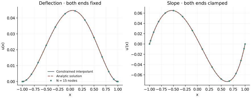
Native GMRES solves the small row-scaled linear system. The displayed solution is \((1-x^2)\) times the interpolant of \(v\), and its slope follows the same product rule. Fitting an ordinary degree-\(N\) polynomial through the solved \(u_j\) would generally lose the clamped slopes between nodes. The book uses monomial fitting for this display; the example uses barycentric evaluation of the same auxiliary polynomial.
An exact solution makes the check decisive
Every solution of \(u^{(4)}=e^x\) is \(e^x\) plus a cubic. Choose the cubic so its values and slopes at both endpoints equal those of \(e^x\). Subtracting it gives the exact clamped solution. The numerical checks solve those four coefficient equations independently and compare every saved value and slope, including both endpoints.
openpfc run model.cpp input.json --source-root .. --launcher=noneresults/beam.csv contains nodal and dense display values, slopes and analytic references. Try degree 8, then 15. Once the smooth forcing is resolved, roundoff and conditioning limit further improvement. This complete-domain polynomial reference runs on one process.
Keep the source, input, clamped-operator helper and collocation helper together.