OpenPFC / Reaction, diffusion and boundaries

Lift the boundary before evolving the interior

A simple function can carry the prescribed endpoint values, leaving a homogeneous quantity for the derivative operator.

Includes the model, inputs, required headers and a short run guide.

Allen–Cahn dynamics combine smoothing with a local preference for two states:

\[ \begin{aligned} u_t&=\epsilon u_{xx}+u-u^3,\\ u(-1,t)&=-1,\quad u(1,t)=1. \end{aligned} \tag{1}\]

For \(\epsilon=.01\), program 34 of Trefethen (2000) begins with \(u(x,0)=.53x+.47\sin(-1.5\pi x)\) and follows its evolution to time 100. Degree 20 is deliberately small enough to inspect the whole model.

Let a line carry the endpoint values

The function \(\ell(x)=x\) already satisfies the two endpoint conditions. Writing \(w=u-\ell\) gives \(w(\pm1)=0\) and \(u_{xx}=w_{xx}\). The full Chebyshev matrix is squared first. Its endpoint rows are then zeroed, so diffusion cannot change those two values. At \(u=\pm1\) the reaction \(u-u^3\) also vanishes.

const auto right_boundary = [](double) { return 1.0; };
return allen_cahn::run(argc, argv, true, right_boundary);

The shared helper keeps the PDE visible and delegates the Euler update to OpenPFC:

const auto rhs = [&](double, const auto &v, auto &dv) {
  auto homogeneous = v;
  if (lifted)
    for (int j = 0; j <= n; ++j) homogeneous[j] -= x[j];
  const auto curvature = polynomial::apply(d2, homogeneous);
  for (int j = 0; j <= n; ++j)
    dv[j] = epsilon * curvature[j] + v[j] - v[j] * v[j] * v[j];
};
pfc::sim::steppers::EulerStepper stepper(dt, u.size(), rhs);

Passing a vector to a native time stepper does not require a uniform physical mesh. The callable owns the spatial interpretation; the stepper only advances an ODE state. Here collocation.hpp supplies an example-owned nonuniform polynomial derivative.

Know which restriction makes an explicit step expensive

Forward Euler uses \(u^{m+1}=u^m+\Delta t\,f(u^m)\). The book chooses

\[ \Delta t=\min(.01,50N^{-4}/\epsilon). \tag{2}\]

The \(N^{-4}\) comes from the large Chebyshev diffusion eigenvalues; compare the grid’s spectrum. The original degree-20 run uses .01. The prescription alone becomes unstable on some finer grids: at degree 40 its diffusive Euler step lies outside the stability region. To make refinement useful, we also calculate \(B=\|(D^2)_{II}\|_\infty\) and cap the step by \(1.8/(\epsilon B+11)\):

double diffusion_bound = 0;
for (int i = 1; i < n; ++i) {
  double row_sum = 0;
  for (int j = 1; j < n; ++j) row_sum += std::abs(d2[i][j]);
  diffusion_bound = std::max(diffusion_bound, row_sum);
}
// |1-3u^2| <= 11 for |u| <= 2; retain a margin below Euler's limit.
const double maximum_dt = std::min({.01, 50.0 / (std::pow(n, 4) * epsilon),
                                    1.8 / (epsilon * diffusion_bound + 11)});

Here 11 bounds \(|1-3u^2|\) for \(|u|\le2\); the factor 1.8 leaves a margin below Euler’s negative-real-axis limit. This diffusion-based guard preserves the original degree-20 timestep and bounds tested refinements; it is not a general nonlinear stability theorem. An explicitly requested step above the cap is rejected. Output-time adjustment cannot increase the step past the cap.

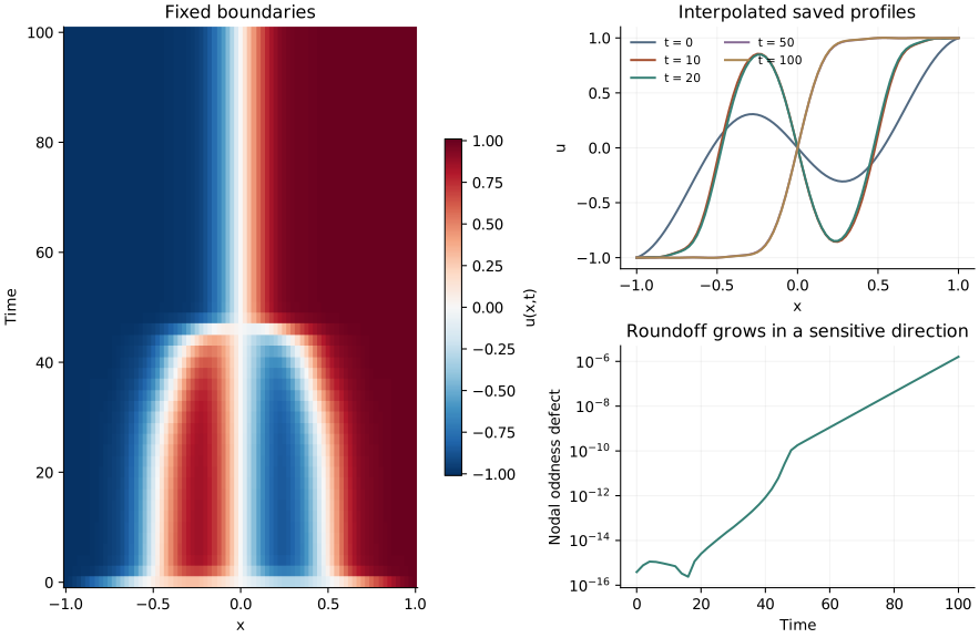
Figure 1: The original fixed-boundary evolution. Profiles at selected times and a nodal symmetry diagnostic accompany the complete saved-time field.

The cubic term drives values toward either \(-1\) or \(1\); diffusion smooths the transition between them. The interfacial scale is proportional to \(\sqrt\epsilon\). A smaller epsilon therefore asks for more spatial resolution, even though it relaxes the diffusive step restriction at a fixed degree.

A symmetric picture can hide a sensitive direction

The exact initial profile is odd. In exact arithmetic the symmetric discrete problem would keep that symmetry. Floating-point evaluation introduces tiny asymmetric components, which this long evolution can amplify. The third panel plots the actual nodal defect \(\max_j|u_j+u_{N-j}|\); its magnitude and sign can vary across platforms. Do not interpret a minute late-time interface displacement as resolved physical symmetry breaking.

This is visible when comparing two independent derivative constructions: their default trajectories agree closely at early times, yet differ by about \(4\times10^{-7}\) at time 100 in the checked CPU run. Restarting the independent calculation from each saved native field separates that accumulated sensitivity from the accuracy of the update. The high-order collocation operator also need not preserve a discrete maximum principle; tiny excursions past \(\pm1\) are possible.

Run, refine and compare

openpfc run model.cpp input.json --source-root .. --launcher=none

results/allen_cahn.csv contains every collocation node and a barycentrically interpolated curve at each saved time. The book fits the same polynomial in a monomial basis for display; barycentric evaluation avoids forming that ill-conditioned representation.

Change epsilon, then vary n and dt separately. Forward Euler has first-order temporal accuracy. Preserving endpoints proves the boundary bookkeeping, but does not prove that an interface is resolved. Tests compare complete small-grid trajectories with independent Lagrange-basis derivatives and check temporal convergence separately.

This is a serial reference with source, input, evolution helper and collocation helper. Continue with a boundary that changes in time.

References

Trefethen, Lloyd N. 2000. Spectral Methods in MATLAB. Society for Industrial; Applied Mathematics. https://doi.org/10.1137/1.9780898719598.