OpenPFC / Reaction, diffusion and boundaries

A changing wall must enter the next derivative

The boundary belongs to the time-dependent state. Updating it at the wrong time changes the problem.

Includes the model, inputs, required headers and a short run guide.

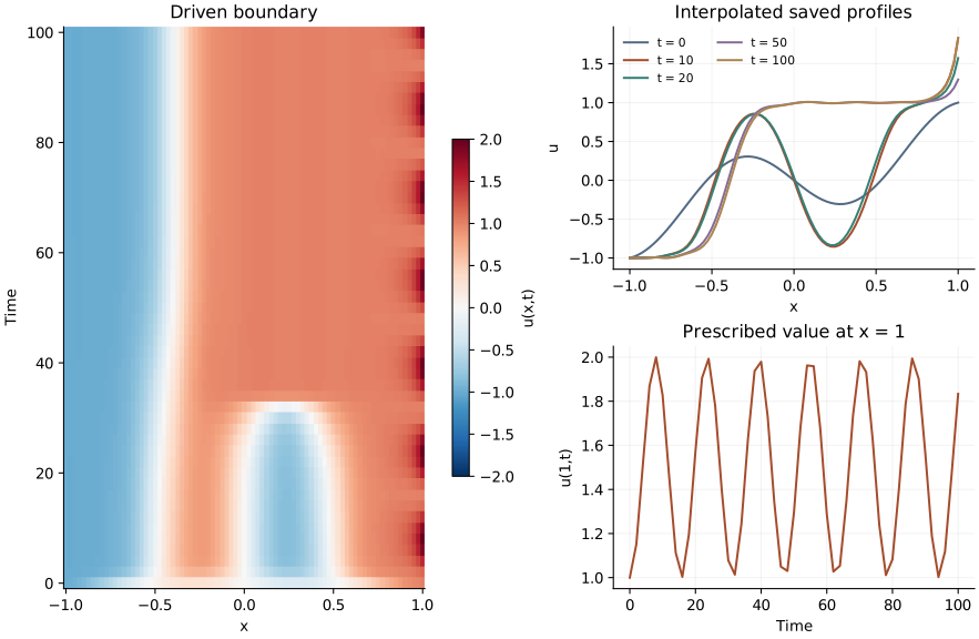
Program 35 of Trefethen (2000) evolves the same Allen–Cahn equation as the fixed-endpoint lesson, but drives one endpoint:

\[ \begin{aligned} u_t&=\epsilon u_{xx}+u-u^3,\\ u(-1,t)&=-1,\\ u(1,t)&=1+\sin^2(t/5). \end{aligned} \tag{1}\]

The upper value lies between 1 and 2. It is prescribed externally; it does not follow the local reaction law. Remember that the Chebyshev samples run from \(x_0=1\) to \(x_N=-1\).

Put the physical boundary in a callable

const auto right_boundary = [](double t) {
  return 1 + std::pow(std::sin(t / 5), 2);
};
return allen_cahn::run(argc, argv, false, right_boundary);

The shared evolution helper uses the full \(D^2\) matrix and the current endpoint values in every interior derivative. In this mode it does not subtract the fixed lift \(x\) or zero the boundary rows. OpenPFC’s Euler stepper forms the provisional next vector, then the two boundary entries are replaced:

for (int step = 1; step <= gap * frames; ++step) {
  stepper.step((step - 1) * dt, u);
  if (!lifted) {
    u.front() = right_boundary(step * dt);
    u.at(n) = -1;
  }
  if (step % gap == 0) observe(step);
}

The overwritten endpoint updates have no influence on that step’s interior values: all right-hand sides were computed from the old state. On the next step, the derivative sees the newly imposed boundary. This is the original program’s explicit method (II).

For a higher-order Runge–Kutta method, imposing a boundary only after the final update would generally be insufficient. Each stage’s interior derivative must see the boundary at its own stage time. This lesson deliberately uses the book’s forward Euler method.

Figure 1: The driven-boundary field and selected interpolated profiles. Values greater than one are the imposed physical boundary, not a plotting overshoot.

Keep the comparison controlled

The default degree, epsilon, initial profile, timestep prescription and saved times match the fixed-boundary experiment. The shared helper keeps the implementation comparable while the two model.cpp files state the different boundary choice.

The default step is .01, with output every 2 time units through time 100. For refinements the operator-based cap also limits the step: the book’s degree-dependent prescription alone can become unstable. The scheduler rounds steps per output interval and increases that count if needed to respect the cap. The CSV reports the actual times. The interpolated curves evaluate the degree-\(N\) polynomial barycentrically, rather than fitting monomial coefficients for display.

openpfc run model.cpp input.json --source-root .. --launcher=none

In results/allen_cahn.csv, verify every saved endpoint against its prescribed value. Then compare dt: .01 with .005: a correct wall does not remove Euler’s first-order interior error. The numerical checks compare the full nodal evolution against independent Lagrange-product second derivatives, including the time-dependent boundary contributions.

The model runs on one process. Keep the source, input, evolution helper and collocation helper together.

References

Trefethen, Lloyd N. 2000. Spectral Methods in MATLAB. Society for Industrial; Applied Mathematics. https://doi.org/10.1137/1.9780898719598.