OpenPFC / Operators and their solutions
A grid has its own spectrum
Distinguish physical Dirichlet eigenmodes from large grid-scale eigenvalues and the timestep restriction they create.
Download runnable lesson (.zip)
Includes the model, inputs, required headers and a short run guide.
A derivative matrix has more to teach than a single derivative. Programs 15 and 26 of Trefethen (2000) examine the Dirichlet problem \(u''=\lambda u\) and the high-frequency end of its Chebyshev discretization. We report the positive eigenvalues of \(-D^2\) so physical frequencies and stiffness can share one graph.
Impose endpoint values before solving an eigenproblem
The full first-derivative matrix is squared before its known-zero boundary values are removed. The interior matrix approximates \(-u''\) on \([-1,1]\). Its continuum eigenvalues are \((j\pi/2)^2\), with corresponding sine modes.
for (int i = 1; i < n; ++i)
  for (int j = 1; j < n; ++j) a[i - 1][j - 1] = -d2[i][j];
const auto pairs = eigen_reference::solve(eigen_reference::complex_matrix(a));
auto spectrum = polynomial::output("spectrum.csv");
spectrum << "mode,eigenvalue,imag,continuum,residual\n";
for (int j = 0; j < n - 1; ++j)
  spectrum << j + 1 << ',' << pairs[j].value.real() << ','
           << pairs[j].value.imag() << ','
           << std::pow((j + 1) * std::numbers::pi / 2, 2) << ','
           << pairs[j].residual << '\n';
The collocation matrix is generally not symmetric in the ordinary Euclidean inner product. The helper therefore uses an example-owned complex shifted QR calculation, rather than applying a symmetric eigensolver to it. It checks every returned eigenpair’s scaled matrix residual. Such a residual measures the finite matrix equation; it cannot establish continuum accuracy.
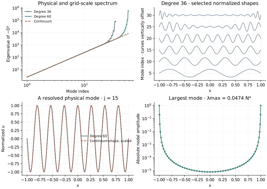
The low modes become spectrally accurate when resolved. Modes near the matrix dimension do not automatically approximate the corresponding continuum sine accurately. Chebyshev endpoint spacing is \(O(N^{-2})\); the largest second-derivative eigenvalues grow as \(O(N^4)\), making an explicit diffusive timestep much more restrictive than on a uniform grid.
Reproduce both experiments
openpfc run model.cpp input.json --source-root .. --launcher=none
openpfc run model.cpp trefethen-p26.json --source-root .. --launcher=none
The first uses degree 36 and modes 5,10,…,30. The second uses degree 60 and shows mode 15 and the largest mode. The original p26 source labels its physical mode N/4 but selects index N/4-1; this preset uses actual mode N/4 and labels it accordingly. Full eigenvalues, imaginary roundoff and scaled residuals are in results/spectrum.csv; nodal and interpolated shapes are in results/modes.csv. modes must stay in 1..n-1.
The tests compare the lowest modes with their exact values and verify all finite eigenpairs against an independently assembled operator. Connect the largest eigenvalue with the stability-region lesson: a stable explicit step is a condition on every resolved discrete mode, not only the physical mode used for an initial condition.
The complete C++ model and starting input are available with this lesson. Keep collocation.hpp in the theme directory. This model also uses eigensystem.hpp in that directory. Download the program 26 preset for the degree-60 experiment.