A hot spot spreads without losing heat

Heat / Follow a whole pulse

A hot spot spreads without losing heat

The peak falls. The width grows. The integral stays put. Check all three against the field.

Download runnable lesson (.zip)

Includes the model, inputs, required headers and a short run guide.

For \(u_t=D\Delta u\) in three-dimensional free space, an initially unit-height Gaussian with width \(\sigma\) evolves as

\[ \begin{gathered} s^2(t)=\sigma^2+2Dt,\\ u_{\mathbb R^3}(\mathbf x,t) =\left(\frac{\sigma}{s(t)}\right)^3 \exp\!\left(-\frac{|\mathbf x|^2}{2s^2(t)}\right). \end{gathered} \]

Substitution verifies the equation. Integrating gives the constant heat \((\sqrt{2\pi}\sigma)^3\). In a large box, this is a useful picture of the early-time pulse. Our FFT, however, solves a periodic problem.

Make the initial condition match the boundary

Periodize the one-dimensional Gaussian by summing its translated images:

\[ G_L(x,t)=\frac{\sigma}{s(t)} \sum_{\ell\in\mathbb Z} \exp\!\left(-\frac{(x+\ell L)^2}{2s^2(t)}\right). \]

The three-dimensional solution is \(u(x,y,z,t)=G_L(x,t)G_L(y,t)G_L(z,t)\). Each term solves heat flow, and the sum has matching values and derivatives at the periodic boundaries. This avoids evolving a truncated free-space Gaussian while comparing it with a different boundary-value problem.

double gaussian_line(double x, double time, const Parameters &p) {
  const double variance = p.width * p.width + 2 * p.diffusivity * time;
  double images = 0;
  for (int image = -12; image <= 12; ++image) {
    const double displacement = x + image * p.length;
    images += std::exp(-displacement * displacement / (2 * variance));
  }
  return p.width / std::sqrt(variance) * images;
}

double exact(double x, double y, double z, double time, const Parameters &p) {
  return gaussian_line(x, time, p) * gaussian_line(y, time, p) *
         gaussian_line(z, time, p);
}

The example retains images \(-12\) through \(12\). It requires \(s^2(t_{\mathrm{final}})\le L^2\), so omitted images are already more than \(12.5\) final widths away at the edge. The discarded tail is negligible at double precision. The image count is an example-specific reference choice, not an OpenPFC boundary condition.

Give the field a callable

Use a periodic grid on \([-L/2,L/2)^3\), with spacing \(L/N\). Field::apply supplies physical coordinates and evaluates the callable only at this process’s owned nodes:

u.apply([&](double x, double y, double z) { return exact(x, y, z, 0, p); });

There is no initializer registry or model inheritance to learn here. The initial-pattern lesson uses the same callable approach for several spatial patterns.

Evolve every resolved Fourier mode

Backward Euler multiplies a mode by \([1+\Delta tD|\boldsymbol\kappa|^2]^{-1}\) at each step. The zero mode therefore stays unchanged. The nonzero modes decay, broadening the pulse.

std::vector<std::complex<double>> modes(fft.size_outbox());
std::vector<double> multiplier(modes.size());
pfc::fft::kspace::for_each_kpoint(
    fft.get_outbox_bounds(), domain,
    [&](std::size_t i, double kx, double ky, double kz, int, int, int) {
      multiplier[i] =
          1 / (1 + p.dt * p.diffusivity * (kx * kx + ky * ky + kz * kz));
    });
for (int step = 0; step < p.steps; ++step) {
  fft.forward(u.vec(), modes);
  for (std::size_t i = 0; i < modes.size(); ++i) modes[i] *= multiplier[i];
  fft.backward(modes, u.vec());
}

The wave-number lesson explains the physical scales and spectral symbols; Trefethen (2000) develops the Fourier differentiation used here. The numerical loop stays separate from the analytic reference and output.

Figure 1: The default native solution along the central grid line, with the periodized analytic pulse. The error panel compares the final numerical and continuum fields on that same line.

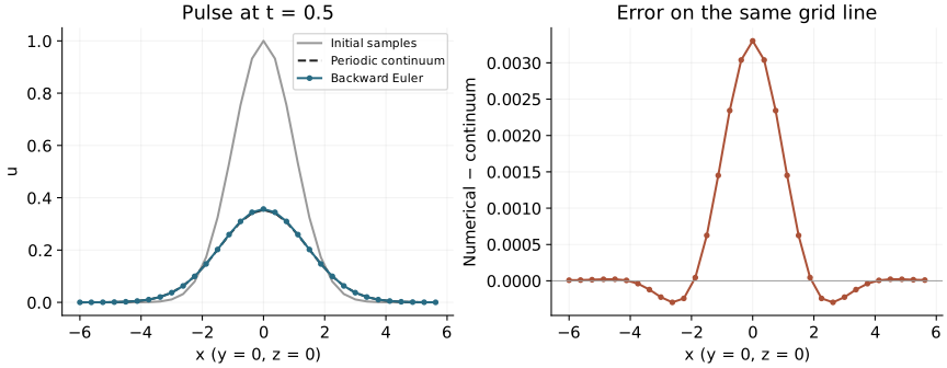
Distinguish two approximation errors

The default run uses \(N=32\), \(L=12\), \(\sigma=1\), \(D=1\), \(\Delta t=0.01\) and 50 steps. It writes each rank’s complete owned field, with initial, numerical and continuum values, plus global mass and error diagnostics.

openpfc run model.cpp input.json
openpfc run model.cpp input.json --ranks=2

Keep the model and input together; neither needs a companion header. Results are under results/ in the CLI attempt directory. Run from one process so that --ranks=2 owns the MPI launch.

Try these two experiments:

1. Keep \(N\) and final time fixed. Halve dt and double steps. Once the pulse is spatially resolved, backward Euler’s error should decrease approximately by a factor of two.
2. Keep the time step fixed and narrow width. The initial peak may then fall between a few widely spaced samples. More time steps cannot recover spatial detail that was never sampled; increase \(N\) as well.

The grid’s conserved quantity is the discrete mass \((L/N)^3\sum_j u_j\). It need not equal the analytic integral when the initial pulse is under-resolved. An unchanged mass alone is therefore insufficient evidence that the field is accurate.

The entry-point checker compares every owned value against independent Fourier-series initialization and direct tensor-product DFT sums. It checks odd/even grids, unique ownership, discrete mass conservation and first-order time refinement on one and two MPI ranks. The displayed reference is checked independently as well. examples/render_utilities.py regenerates the figure from native field CSVs.

References

Trefethen, Lloyd N. 2000. Spectral Methods in MATLAB. Society for Industrial; Applied Mathematics. https://doi.org/10.1137/1.9780898719598.