Fourier / Give a mode its units
An FFT index is not a wave number
Change the length of the domain. The array indices stay put; the derivatives change.
Download runnable lesson (.zip)
Includes the model, inputs, required headers and a short run guide.
On a periodic interval of length \(L\), the integer mode \(m\) represents \(\exp(i\kappa_m x)\) with \(\kappa_m=2\pi m/L\). Its first derivative has multiplier \(i\kappa_m\); its second derivative has multiplier \(-\kappa_m^2\). This is the Fourier differentiation viewpoint of Trefethen (2000).
Start with the physical box
The default grid has \(8\times9\times6\) points and lengths \((2\pi,3\pi,\pi)\). Periodic spacing is \(L/N\): the endpoint is not a second copy of the origin.
const auto domain = pfc::domain::create(
    pfc::GridSize{shape}, pfc::PhysicalOrigin{{0, 0, 0}},
    pfc::GridSpacing{
        {length[0] / shape[0], length[1] / shape[1], length[2] / shape[2]}});
const auto scale = pfc::fft::kspace::k_frequency_scaling(domain);
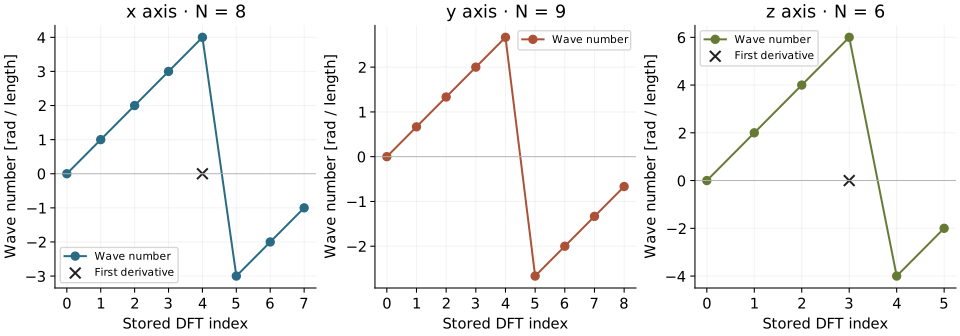
The three frequency scales are \(1\), \(2/3\) and \(2\) radians per unit length. The same integer mode therefore describes different derivatives on each axis.
Read the stored order deliberately
For \(N=8\), OpenPFC labels the full DFT indices by modes \(0,1,2,3,4,-3,-2,-1\). The even-grid Nyquist label is positive. For \(N=9\), the labels are \(0,1,2,3,4,-4,-3,-2,-1\); there is no Nyquist sample.
const double k =
    pfc::fft::kspace::k_component(index, shape[axis], scale[axis]);
const double k_odd =
    pfc::fft::kspace::k_component_odd(index, shape[axis], scale[axis]);
const double laplacian = pfc::fft::kspace::k_laplacian_value(k, 0, 0);
The odd-derivative component sets the even-grid Nyquist wave number to zero. Indeed, \(\cos(\pi j)=(-1)^j\) samples a Nyquist cosine with \(\kappa_{\mathrm{Ny}}=\pi N/L\), whose first derivative vanishes at these nodes. Its second derivative does not vanish:
\[ \begin{gathered} \left.\frac{d}{dx}\cos(\kappa_{\mathrm{Ny}}x)\right|_{x_j}=0,\\ \left.\frac{d^2}{dx^2}\cos(\kappa_{\mathrm{Ny}}x)\right|_{x_j} =-\kappa_{\mathrm{Ny}}^2(-1)^j. \end{gathered} \]
Consequently, applying the nodal first derivative twice does not recover the direct second derivative of this mode. Keep k_component for the Laplacian; use k_component_odd for an ordinary first derivative of a real field. More general tensor operators need their own Hermitian-symmetry argument; this lesson does not supply one.
Build an operator from its symbol
For heat flow \(u_t=\Delta u\), each Fourier coefficient solves \(\widehat u_t=\lambda\widehat u\), with \(\lambda=-(\kappa_x^2+\kappa_y^2+\kappa_z^2)\). Backward Euler and exact linear evolution use different multipliers:
\[ \begin{gathered} g_{\mathrm{BE}}=\frac{1}{1-\Delta t\lambda},\\ g_{\mathrm{exact}}=\exp(\Delta t\lambda). \end{gathered} \]
pfc::fft::kspace::for_each_kpoint(
    box, domain,
    [&](std::size_t offset, double kx, double ky, double kz, int i, int j,
        int k) {
      const double lap = pfc::fft::kspace::k_laplacian_value(kx, ky, kz);
      const double implicit = 1 / (1 - dt * lap);
      const double exponential = std::exp(dt * lap);
      symbols << offset << ',' << i << ',' << j << ',' << k << ',' << kx << ','
              << ky << ',' << kz << ',' << lap << ',' << implicit << ','
              << exponential << '\n';
    });
The zero mode has multiplier one: heat flow preserves the mean. For nonzero modes, \(0<g_{\mathrm{exact}}<g_{\mathrm{BE}}<1\). An unconditionally stable step can still damp too slowly. The implicit heat lesson applies the backward-Euler multiplier to an actual distributed FFT.
Here box is the complete x-compressed real-to-complex box. This small program inspects symbols without allocating or executing an FFT. A distributed solver instead passes its rank’s actual outbox to the same iterator; the callback offset then indexes that rank’s spectrum.
Change one length
openpfc run model.cpp input.json --launcher=noneThe model and input need no companion header. The run writes results/axes.csv and results/symbols.csv in its attempt directory. Double every length and run again: each wave number halves, and each Laplacian eigenvalue becomes one quarter of its former value. Then change an even point count to an odd one and predict which zero in the odd-derivative table will disappear.
The entry-point checker checks every symbol on mixed-parity, odd and rescaled boxes against independently enumerated physical Fourier basis functions. It also checks the compressed-box ownership, mean multiplier and invalid inputs. The figure comes from the default native CSV table; examples/render_utilities.py regenerates it.