OpenPFC / From an equation to a field

Write an initial condition as a function

Define the pattern in physical space. Let the field visit the samples owned by this rank.

Includes the model, inputs, required headers and a short run guide.

An initial condition is a function evaluated at grid coordinates. It need not know how many MPI ranks hold the field or which local array offset corresponds to a point. This refactoring of 14_custom_field_initializer turns its Gaussian, vortex and checkerboard demonstrations into actual owned-field output, rather than separate printed samples of the formulas.

Keep parameters in a small callable

The Gaussian has width \(\sigma\) and unit height:

\[ g(\mathbf x)=\exp[-|\mathbf x|^2/(2\sigma^2)]. \tag{1}\]

struct Gaussian {
  double width;
  double operator()(double x, double y, double z) const {
    return std::exp(-(x * x + y * y + z * z) / (2 * width * width));
  }
};

field.apply(Gaussian{width}) fills the field. The object carries its width, so the function needs no global variable. The default grid is a z=0 slice of a three-dimensional pattern; increasing nz samples a slab over \(0\le z<1\). Both descriptions use the same callable.

Treat a removable singularity explicitly

A regularized vortex has tangential speed

\[ \begin{gathered} v_\theta(r)=\frac{\Gamma}{2\pi r}(1-e^{-r^2/a^2}), \\ v_\theta(0)=0. \end{gathered} \tag{2}\]

field.apply([&](double x, double y, double) {
  const double r = std::hypot(x, y);
  return r == 0 ? 0
                : -circulation * std::expm1(-r * r / (core * core)) /
                      (2 * std::numbers::pi * r);
});

Near zero, \(v_\theta\sim\Gamma r/(2\pi a^2)\). expm1 evaluates \(e^z-1\) accurately when \(z\) is small. The explicit centre case avoids division by zero. This field stores a scalar tangential speed; it is not a two-component velocity field or an evolved fluid solution.

A discontinuity is also a legitimate initial field

field.apply([](double x, double y, double z) {
  const int cell =
      static_cast<int>(std::floor(x) + std::floor(y) + std::floor(z));
  return cell % 2 ? -1.0 : 1.0;
});

The unit cells are defined by floor of physical coordinates, including negative coordinates. Rank-local indices would move the pattern when the partition changed. Its sharp jumps also explain why Fourier derivatives of such data need more care than derivatives of a smooth Gaussian.

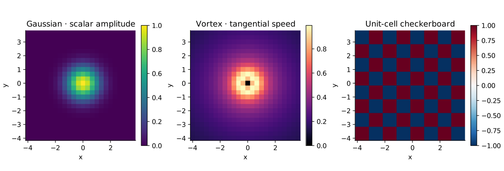
Figure 1: The three actual initial fields on the default z=0 slice. Each panel has its own units and colour scale.

Fill once, inspect everywhere

openpfc run model.cpp input.json --source-root .. --launcher=none
openpfc run model.cpp input.json --source-root .. --ranks=2 --launcher=mpirun

Each rank writes its owned samples to results/fields_rank_*.csv. The checks reconstruct the complete grid and compare every value with the three formulas on one and two ranks. These are prescribed patterns; the Gaussian and vortex tails are not made periodic by the grid metadata.

Change width, core or circulation. Then increase n and decide which features are resolved. To select a pattern by name in a file, continue with the modifier catalog. Keep the source, input and shared helper together.