Use polar coordinates to define a Cartesian field

OpenPFC / A small callable carries the mathematics

Use polar coordinates to define a Cartesian field

Describe a pattern in the coordinates that make its structure clear, then let OpenPFC evaluate it at owned Cartesian points.

Download runnable lesson (.zip)

Includes the model, inputs, required headers and a short run guide.

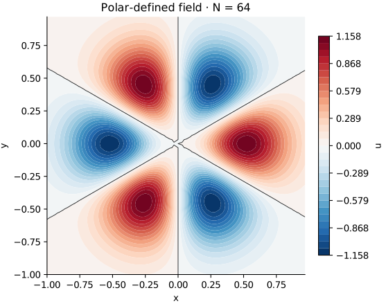
A Gaussian has a radial envelope. Give it an angular harmonic and it develops a recognizable lobe pattern:

\[ u(r,\theta)=\left(\frac{r}{\sigma}\right)^m e^{-r^2/(2\sigma^2)}\cos(m\theta). \tag{1}\]

The default uses \(m=3\) and \(\sigma=0.3\). The grid samples the Cartesian square \([-1,1)^2\), with spacing \(2/N\). Each MPI rank initializes only the points that it owns.

Give a point another interpretation

An ordinary C++ function maps a Cartesian point to radius and angle:

struct Polar {
  double radius, angle;
};

Polar polar(double x, double y) {
  const double r = std::hypot(x, y);
  return {r, r == 0 ? std::numeric_limits<double>::quiet_NaN() : std::atan2(y, x)};
}

atan2 handles all quadrants. At the origin the angle is undefined; the mapping records NaN instead of pretending there is a preferred direction. The physical scalar field still has a well-defined limit.

Put the continuous limit into the callable

struct AngularGaussian {
  double width;
  int harmonic;

  double operator()(double x, double y, double) const {
    const auto [r, theta] = polar(x, y);
    if (r == 0) return harmonic == 0 ? 1 : 0;
    return std::pow(r / width, harmonic) * std::exp(-r * r / (2 * width * width)) *
           std::cos(harmonic * theta);
  }
};

For \(m>0\) the factor \(r^m\) makes the centre value zero. For \(m=0\) the field is the usual Gaussian, whose centre value is one. Both cases are smooth because Equation 1 can also be written

\[ \begin{aligned} u(x,y)&=\operatorname{Re} \left[\left(\frac{x+iy}{\sigma}\right)^m\right]\\ &\quad\times e^{-(x^2+y^2)/(2\sigma^2)}. \end{aligned} \tag{2}\]

For example, the cubic factor at \(m=3\) is \((x^3-3xy^2)/\sigma^3\). This independent Cartesian formula supplies the numerical check without reusing the C++ polar evaluator.

The angle jumps at its branch cut, but the integer angular harmonic gives the same scalar field on both sides. Removing the radial factor would also remove the continuous centre limit for nonzero \(m\).

Let the native field evaluate the expression

const auto domain = pfc::domain::create(
    pfc::GridSize{{n, n, 1}}, pfc::PhysicalOrigin{{-1, -1, 0}},
    pfc::GridSpacing{{2.0 / n, 2.0 / n, 1}}, pfc::Bool3{false, false, false});
const auto partition = pfc::decomposition::create(domain, comm.size());
auto field = pfc::data::field_from_subdomain<double>(partition, comm.rank(), 0);
field.apply(AngularGaussian{width, harmonic});

The callable is the extension point used here. The domain, ownership boxes and differential operators keep their Cartesian meaning. To solve a differential equation in polar coordinates, follow the disk-mode and polar Poisson chapters, which derive and apply the corresponding operator.

Figure 1: The default three-fold angular pattern on the actual Cartesian field. Positive and negative lobes meet smoothly at the origin; the Cartesian alternative is the same function.

Experiment on one process, then two

openpfc run model.cpp input.json --launcher=none
openpfc run model.cpp input.json --ranks=2 --launcher=mpirun

Each attempt writes results/polar_rank_<rank>.csv, containing global indices, physical points, polar coordinates and the owned scalar values. The undefined angle is the only nonfinite output, at the origin when the grid contains it. The scalar values there are finite.

Try harmonic: 0, then 1 and 3, retaining JSON’s quotes around the key. Predict the number and signs of the lobes. Change width without changing the grid. Then compare one and two ranks: the ownership changes, while the same Cartesian formula determines every global point. An odd grid such as \(N=9\) omits the origin; compare its samples with an even grid that includes it.

The checks assemble complete owned fields, reject duplicate or missing points, verify the origin limits, and compare four parameter choices with the complex-polynomial formula. Keep the source and input together. The model accepts \(N\) from 8 through 128, integer harmonics 0 through 8 and widths 0.05 through 1. This refactors the earlier coordinate-wrapper demonstration while retaining its 17_custom_coordinate_system executable name.