OpenPFC / Fourier modes meet polar geometry
Meet at the centre of a disk
The centre is shared by every angle. A half-turn connects the two signs of the radial coordinate.
Download runnable lesson (.zip)
Includes the model, inputs, required headers and a short run guide.
Program 28 of Trefethen (2000) finds vibration modes of a unit disk:
\[ -\Delta u=\lambda u,\qquad u(1,\theta)=0. \tag{1}\]
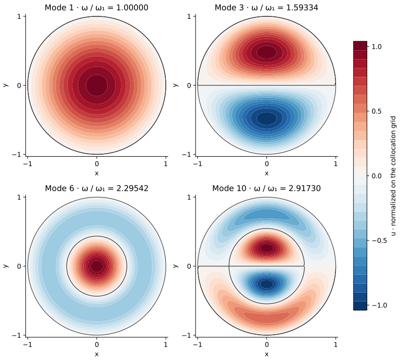
For the unit-speed wave equation, \(\lambda=\omega^2\). The book displays four shapes, with sorted indices 1, 3, 6 and 10, and reports their frequencies relative to the fundamental.
In polar coordinates,
\[ \Delta u=u_{rr}+\frac{u_r}{r}+\frac{u_{\theta\theta}}{r^2}. \tag{2}\]
The coefficients look singular at the centre. Start with the geometry before dividing by the radius.
Give negative radius a geometric meaning
The points \((-r,\theta)\) and \((r,\theta+\pi)\) represent the same Cartesian point. For an angular Fourier mode \(e^{ik\theta}\) this gives
\[ R_k(-r)=(-1)^kR_k(r). \tag{3}\]
Use an odd degree \(N\) for the signed Lobatto grid on \([-1,1]\). There is no node at zero, and each positive radial unknown has a negative partner. The default \(N=25\) leaves twelve positive interior radii. Both boundary radii have zero value.
Native OpenPFC derivatives supply the complete one-dimensional matrices:
r = pfc::fft::chebyshev_lobatto(n);
first.assign(n + 1, Vector(n + 1));
Vector unit(n + 1);
for (int j = 0; j <= n; ++j) {
  unit.at(j) = 1;
  const auto column = pfc::fft::chebyshev_derivative(unit);
  for (int i = 0; i <= n; ++i) first[i][j] = column[i];
  unit[j] = 0;
}
second = polynomial::square(first);
The complete matrices are formed before selecting interior equations. With \(\partial_{\theta\theta}=-k^2\), fold the negative columns into the positive ones using Equation 3:
const double parity = k % 2 ? -1 : 1;
for (int i = 1; i <= radial; ++i)
  for (int j = 1; j <= radial; ++j) {
    a[i - 1][j - 1] = second[i][j] + first[i][j] / r[i] +
                      parity * (second[i][n - j] + first[i][n - j] / r[i]);
    if (i == j) a[i - 1][j - 1] -= k * k / (r[i] * r[i]);
  }
This is an example-owned polar composition. Native Chebyshev differentiation and the local FFT are public OpenPFC building blocks; the helper does not introduce a production polar-grid backend.
Preserve the multiplicity of an angular mode
The book diagonalizes one \(240\times240\) tensor matrix at \(N=25\), \(M=20\). Fourier separation gives the same matrix spectrum through eleven small radial blocks. For each nonzero frequency below Nyquist, cosine and sine give two independent shapes with the same eigenvalue:
for (int k = 0; k <= grid.m / 2; ++k) {
  auto a = grid.laplacian(k);
  for (auto &row : a)
    for (auto &value : row) value = -value;
  const auto radial_modes =
      eigen_reference::solve(eigen_reference::complex_matrix(a));
  for (int j = 0; j < grid.radial; ++j) {
    modes.push_back({radial_modes[j], k, j + 1, false});
    if (k != 0 && k != grid.m / 2)
      modes.push_back({radial_modes[j], k, j + 1, true});
  }
}
The zero mode and the angular Nyquist mode each have one real sampled shape. Keeping those multiplicities gives all 240 eigenvalues. It also chooses a reproducible orientation inside a repeated eigenspace; a rotated linear combination of a sine/cosine pair describes an equally valid mode.
Reconstruct the centre deliberately
The plotted radial polynomial uses the signed nodal values and their Fourier parity:
const polynomial::Interpolant interpolate(
    grid.r, disk::extend(grid, positive, mode.k));
const auto observe = [&](const char *kind, int ir, int it, double r,
                         double theta) {
  const double value =
      r == 0 && mode.k != 0 ? 0 : interpolate(r) * angular(theta);
  fields << index << ',' << kind << ',' << ir << ',' << it << ',' << r << ','
         << theta << ',' << r * std::cos(theta) << ',' << r * std::sin(theta)
         << ',' << value << '\n';
};
The original collocation grid has no pole unknown. For the display, the axisymmetric mode takes its interpolated value at zero; nonzero angular modes use the regular limit zero. The display grid adds no PDE resolution. Normalization uses the largest absolute collocation value, so an interpolated value between nodes can slightly exceed one.
Parity alone is not a complete regularity condition for every angular mode. Check the selected low modes against their continuum forms:
\[ \begin{aligned} u(r,\theta)&=J_k(\alpha r) \begin{cases}\cos(k\theta),\\\sin(k\theta),\end{cases}\\ J_k(\alpha)&=0. \end{aligned} \tag{4}\]
The positive Bessel zeros and their notation are described in National Institute of Standards and Technology (n.d.). Their squares give the eigenvalues; the zeros themselves give frequency ratios. The independent numerical check evaluates Bessel series and brackets their roots, then compares all saved nodal and display values of the four selected shapes. It also checks every discrete radial eigenvector and the full polar action, including the angular derivative.
Run the original experiment
openpfc run model.cpp input.json --source-root .. --launcher=noneThe input retains the book’s \(N=25\), \(M=20\). The output includes every eigenvalue in results/spectrum.csv, every radial eigenvector with its angular labels in results/radial.csv, the four frequency ratios in results/selected.csv, and all plotted fields in results/fields.csv. The picture uses a two-dimensional field and nodal lines in place of the book’s wireframe projection.
Try \(N=15\), then 25. Compare eigenvalues and shape errors before judging the smoothness of a plot. Then increase \(M\): predict which angular modes become representable and which low modes should remain unchanged. Continue with Poisson’s equation on the same disk to separate geometry from the regularity of the forcing.
This complete-domain reference uses one process, odd degrees 7 through 63 and even angular counts 8 through 64. Keep the model, polar helper, eigensolver and collocation helper together.