A small residual can leave a visible error

OpenPFC / Geometry, forcing and convergence

A small residual can leave a visible error

Solve the collocation equations accurately. Then ask how accurately they represent the continuous problem.

Download runnable lesson (.zip)

Includes the model, inputs, required headers and a short run guide.

Program 29 of Trefethen (2000) solves \(\Delta u=f\) on the unit disk, with \(u=0\) at \(r=1\). Its forcing is

\[ \begin{aligned} f(r,\theta)&=-r^2\sin^4(\theta/2)\\ &\quad+\sin(6\theta)\cos^2(\theta/2). \end{aligned} \tag{1}\]

Reuse the signed-radius operator from the disk-mode chapter. The book’s \(N=31\), \(M=40\) grid has fifteen positive interior radii and 600 unknowns. Angular Fourier separation turns the full matrix solve into small radial solves.

Keep the physical forcing visible

const auto source = [manufactured](double r, double theta) {
  return manufactured
             ? -4 - 8 * r * std::cos(theta) - 3 * r * r * std::cos(2 * theta)
             : -r * r * std::pow(std::sin(theta / 2), 4) +
                   std::sin(6 * theta) * std::pow(std::cos(theta / 2), 2);
};

The optional manufactured case supplies a smooth Cartesian polynomial. Begin with the original forcing and transform each radial ring using OpenPFC’s native complete-domain FFT:

for (int j = 0; j < grid.radial; ++j) {
  for (int t = 0; t < grid.m; ++t)
    forcing[t + grid.m * j] = line[t] = source(grid.r[j + 1], grid.angle(t));
  fft.forward(line, coefficients[j]);
}

The samples are at \(\theta_j=2\pi(j+1)/M\), matching the book. The transform works on array indices; reconstruction therefore uses \(e^{ik(\theta-2\pi/M)}\). Keeping that phase convention preserves the physical orientation of the field.

Solve each real radial system with native GMRES

for (int k = 0; k <= grid.m / 2; ++k) {
  const auto a = grid.laplacian(k);
  disk::Vector real_rhs(grid.radial), imaginary_rhs(grid.radial);
  for (int j = 0; j < grid.radial; ++j) {
    real_rhs[j] = coefficients[j][k].real();
    imaginary_rhs[j] = coefficients[j][k].imag();
  }
  const auto real = polynomial::solve(a, real_rhs);
  const auto imaginary = polynomial::solve(a, imaginary_rhs);
  for (int j = 0; j < grid.radial; ++j)
    coefficients[j][k] = disk::Complex(real[j], imaginary[j]);
}
for (int j = 0; j < grid.radial; ++j) {
  fft.backward(coefficients[j], line);
  for (int t = 0; t < grid.m; ++t) u[t + grid.m * j] = line[t];
}

The radial operator is real. Its real and imaginary right-hand sides use the same row-scaled native GMRES solve. The forward FFT is unscaled and the backward FFT divides by \(M\), so retaining those coefficients through the radial solves gives the correct physical amplitude. Every represented angular mode is retained; there is no smoothing or deliberate filtering.

The model then checks the original polar equations through the full radial/half-turn action and a native angular second derivative. A small residual establishes that these discrete equations were solved. An exact solution lets us ask a different question about the approximation.

Figure 1: The book’s computed Poisson field and its difference from the exact separated solution. The error panel uses its own much smaller scale.

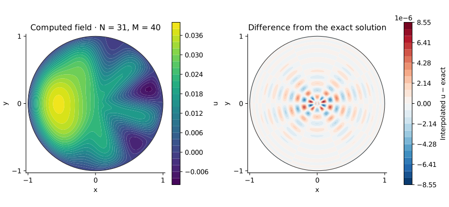
The picture interpolates the computed modal coefficients onto a display grid. Its smooth appearance adds no PDE unknowns; the error panel compares that interpolated field with the exact solution at the display points.

Derive an exact reference by separating the forcing

For a sine or cosine angular factor of order \(k\),

\[ \Delta\bigl(r^p e^{ik\theta}\bigr) =(p^2-k^2)r^{p-2}e^{ik\theta}. \tag{2}\]

A term \(c r^q\) in the forcing therefore has the zero-boundary particular solution

\[ u_k(r)=c\,\frac{r^{q+2}-r^k}{(q+2)^2-k^2}, \tag{3}\]

provided the denominator is nonzero. The subtracted \(r^k\) is harmonic. Expanding the original forcing gives six terms:

Angular factor	Forcing amplitude	Solution amplitude
\(1\)	\(-3r^2/8\)	\(3(1-r^4)/128\)
\(\cos\theta\)	\(r^2/2\)	\((r^4-r)/30\)
\(\cos2\theta\)	\(-r^2/8\)	\((r^2-r^4)/96\)
\(\sin6\theta\)	\(1/2\)	\((r^6-r^2)/64\)
\(\sin5\theta\)	\(1/4\)	\((r^5-r^2)/84\)
\(\sin7\theta\)	\(1/4\)	\((r^7-r^2)/180\)

Multiplying and summing the last column gives a continuous zero-boundary solution, with centre value \(3/128\). The numerical check reconstructs it from the general power formula rather than copying the model’s closed expression.

The forcing is not smooth at the centre

The term \(\sin(6\theta)\cos^2(\theta/2)\) has different limits along different rays as \(r\to0\). There is no unique forcing value at that point. The collocation grid omits the pole; the display evaluates the regular axisymmetric limit of the solution there.

In particular, odd angular modes in this solution contain positive-radius \(r^2\) terms. Their signed odd extensions behave as \(r|r|\) near zero and are not analytic. These terms limit radial polynomial convergence. Other terms are exactly representable radial polynomials, so the regularity question concerns the representation as well as Cartesian smoothness.

At the default grid the largest nodal solution error is about \(6.9\times10^{-7}\) while the largest equation residual is about \(5.9\times10^{-13}\). The radial refinement input raises \(N\) to 63 at the same \(M=40\) and reduces the nodal error to about \(1.3\times10^{-7}\). These are errors against the exact continuous solution; a tiny discrete residual alone cannot show them. The interpolated display reaches a larger error, about \(8.6\times10^{-6}\), between the two innermost collocation rings at \(r\approx0.094\). The error panel therefore reveals reconstruction behaviour between the solved nodes as well as the error at those nodes. With \(N=63\), the same display grid has a largest error of about \(2.0\times10^{-6}\).

Manufacture a smooth answer before changing the model

The manufactured input uses

\[ \begin{aligned} u&=(1-x^2-y^2)\\ &\quad\times\bigl[1+x+\tfrac14(x^2-y^2)\bigr],\\ f&=-4-8x-3(x^2-y^2). \end{aligned} \tag{4}\]

The field is a degree-four Cartesian polynomial with zero boundary values. The degree-15 radial, 16-angle case reproduces it near roundoff; this isolates the operator and normalization checks from the book forcing’s radial approximation error.

openpfc run model.cpp input.json --source-root .. --launcher=none
openpfc run model.cpp manufactured.json --source-root .. --launcher=none
openpfc run model.cpp refine-radius.json --source-root .. --launcher=none

Each preserved attempt writes results/solution.csv with the full nodal field, dense display samples and exact reference, plus results/diagnostics.csv with the equation residual and nodal error. Try refining the angular count alone: once these seven Fourier modes are resolved, that change cannot remove the radial error. Then replace the forcing by a smooth Cartesian harmonic and derive its particular solution.

This complete-domain reference runs on one process. Keep the model, input, polar helper and collocation helper together. Use odd \(N\) from 7 through 63 and even \(M\) from 8 through 64; the book forcing requires \(M\ge16\) to resolve its angular content.

References

Trefethen, Lloyd N. 2000. Spectral Methods in MATLAB. Society for Industrial; Applied Mathematics. https://doi.org/10.1137/1.9780898719598.