
Introduction
Tungsten is used where materials must endure extreme conditions. Making a sound component, however, requires more than selecting a refractory metal: solidification leaves a grain structure, and the interfaces between grains influence the resulting material. Studies of laser-manufactured tungsten identify solidification cracking and embrittling grain-boundary features as practical obstacles1.
Phase-field crystal (PFC) modelling asks how crystalline order develops in a continuous density field. Its periodic peaks retain lattice-scale structure while the field evolves on diffusive timescales2. This places PFC between a conventional continuum phase-field description and trajectories of individual atoms. Its connection to density functional theory helps explain how crystal orientations, strain, and defects can arise in the field3.
The question
What happens when differently oriented BCC nuclei grow in the same undercooled melt? Where does order develop, and what remains disordered when grains meet?
PFC literature demonstrates a broad range of defect physics4. The calculation discussed here tests grain growth within the current OpenPFC model. It does not establish a manufacturing prediction or experimental validation. The OpenPFC paper provides the published model family and rapid-solidification context5.
Governing equations
The state variable is the reduced density field \(\psi(\mathbf{x},t)\). A nearly uniform field represents disordered matter; an oscillatory field represents crystalline order. The density peaks are a coarse-grained representation, rather than moving particles. In reduced units, the conserved PFC evolution is
\[ \frac{\partial\psi}{\partial t} =\nabla^2\frac{\delta F}{\delta\psi}. \tag{1}\]
The Laplacian makes the spatial mean constant in a periodic domain with no external field modifiers. A density reservoir changes that balance, even though the FFT domain remains periodic.
A useful free-energy organization is
\[ F[\psi]=\int\left[ \frac12\psi C(\nabla^2)\psi +f_{\mathrm{loc}}(\psi,\psi_{\mathrm{MF}}) \right]\,d\mathbf{x}. \tag{2}\]
Here \(C\) collects the quadratic correlation and density response, while the remainder contains nonlinear density and mean-field terms. The argument \(\psi_{\mathrm{MF}}\) is a filtered version of \(\psi\), so “local” refers to pointwise evaluation after filtering, rather than a completely local functional of \(\psi\). To specify what the current code actually evolves, it is clearest to give its chemical-potential split explicitly.
Correlation, filtering, and lattice selection
Let \(k=|\mathbf{k}|\), \(u=-k^2\), and \(\kappa=k-1\). The implemented symbols are
\[ \widehat\psi_{\mathrm{MF}}=\chi(k)\widehat\psi, \qquad \chi(k)=\exp\!\left(-\frac{k^2}{2\lambda^2}\right), \tag{3}\]
\[ C_s(k)=s+\bar p_2-B_x e^{-T/T_0}g(\kappa)+\bar q_2\chi(k). \tag{4}\]
For the fourth-order peak used by the shipped Tungsten parameters,
\[ g(\kappa)=\begin{cases} \exp\!\left[-\dfrac{\kappa^2+r_{\mathrm{tol}}\kappa^4}{2\alpha^2}\right], &\kappa<0,\\[4pt] 1-\dfrac{\kappa^2}{2\alpha^2},&\kappa\geq0, \end{cases} \tag{5}\]
where \(r_{\mathrm{tol}}=-2\alpha^2\log(\alpha_{\mathrm{farTol}})-1\). The correlation peak selects \(k_0=1\), giving a radial lattice period of \(2\pi\) in reduced length units. BCC order is initialized with the six \(\{110\}\) density-wave directions. The peak sets the wavelength; its interaction with the nonlinear terms stabilizes the crystalline state.
The filter in Equation 3 suppresses lattice oscillations in the mean-field density. Its long-wavelength terms control the bulk density response. Temperature enters the peak through \(e^{-T/T_0}\) and enters the transformed polynomial coefficients. The bars denote the coefficient transformation used by the Tungsten parameterization, including its density shift.
The nonlinear response and thermal drive
The pointwise nonlinear term used by the current implementation is
\[ \begin{aligned} N(\psi,\psi_{\mathrm{MF}})={}&-s\psi +\bar p_3\psi^2+\bar p_4\psi^3\\ &+\bar q_3\psi_{\mathrm{MF}}^2 +\bar q_4\psi_{\mathrm{MF}}^3. \end{aligned} \tag{6}\]
Thus the evolved chemical potential is \(C_s\psi+N\). The numerical stabilizer \(s\) is added in Equation 4 and subtracted in Equation 6; it changes the time-integration split without changing the combined right-hand side. These expressions follow the current spectral physics and pointwise response.
An optional drive prescribes \(T_{\mathrm{loc}}(x,t)=T+G(x'-x_0-Vt)\), with \(x'\) unwrapped using the tracked front. The current pointwise response then rebuilds \(\bar q_3=\bar q_{30}+\bar q_{31}T_{\mathrm{loc}}/T_0\); the linear peak remains at the reference \(T\). This is a prescribed coefficient field, not a solved heat-transfer equation. No drive is used in the closed case.
Numerical method
OpenPFC samples the field on a periodic structured grid and represents spatial derivatives in Fourier space. In that representation, Equation 1 becomes
\[ \partial_t\widehat\psi =L(k)\widehat\psi+u\widehat N, \qquad L(k)=uC_s(k),\quad u=-k^2. \tag{7}\]
Both channels carry the conserving \(-k^2\) factor. At \(k=0\) it vanishes, so a closed calculation preserves the zero mode. The linear response is handled exponentially, while the nonlinear response is evaluated from the current real-space field. First-order exponential time differencing gives
\[ \widehat\psi^{\,n+1} =e^{L\Delta t}\widehat\psi^{\,n} +\Delta t\,\varphi_1(L\Delta t)\,u\widehat N^{\,n}, \qquad \varphi_1(z)=\frac{e^z-1}{z},\quad\varphi_1(0)=1. \tag{8}\]
FFTs connect the two representations, including the filtered density. HeFFTe distributes the transforms across MPI ranks. CPU, CUDA, and HIP variants use the same model symbols and nonlinear response when the corresponding FFT backend is configured. ETD treats the stiff linear response efficiently; it does not remove spatial-resolution or timestep error.
Simulation setup
The designed reference experiment is a genuinely three-dimensional polycrystal: 64 differently oriented BCC seeds in a closed, isothermal melt. The chosen spacing resolves eight grid points per radial lattice period. It follows the resolution comparison in Section 7 rather than the coarser shipped demonstration presets.
| Quantity | Reference configuration |
|---|---|
| Domain | Periodic cube, \([0,128\pi)^3\) in reduced length units |
| Grid | \(512^3\) cells; \(\Delta x=\Delta y=\Delta z=\pi/4\) |
| Time integration | ETD1, \(\Delta t=1\) reduced time unit |
| Seeds | \(4\times4\times4\), radius 28, amplitude 0.215936, density −0.047 |
| Orientations | Random Euler angles; deterministic generator seed 42 |
| Melt | Initially \(\psi=0\) outside the seeds |
| Temperature | Reference \(T=3300\), \(T_0=156000\); no prescribed drive |
| Reservoir | None; no fixed or moving density modifier |
| Execution | HIP / HeFFTe, eight MI250X GCDs, one LUMI-G node |
| Output | Full density field every 100 time units |
The initial melt has \(\psi=0\). The model reference parameter \(n_0=-0.10\) is distinct from this initial field value.
The initial centers are jittered by up to 20% of the seed radius. The periodic cube permits grains to encounter neighbors across all faces; those faces are not container walls. Length and time are reported in reduced units. A physical conversion is not inferred from the paper without a parameter-by-parameter calibration check.
The scientific stop criterion requires impingement and a stable late-time window in bulk order and spectral observables. A scheduled time cap alone is not evidence that this criterion has been met.
Simulation results
The new \(512^3\) showcase awaits execution and admission against the stop criterion. Its fields and derived figures will be admitted here after numerical and provenance checks. The earlier thin-slab images are not substituted for a three-dimensional result.
Quantitative analysis
The closed case requires four complementary diagnostics: ordered volume, first-shell spectral power, disordered volume, and the spatial mean density. An amplitude threshold must be varied to show how the ordered-volume estimate depends on classification. A low-amplitude fraction includes both residual melt and grain-boundary cores; it cannot be called a grain-boundary fraction before impingement is established.
These measurements separate the emergence of a lattice from the growth of its occupied volume. Conservation tests a distinct numerical property. No free-energy curve is shown: a diagnostic assembled from a guessed functional would not test this implementation.
Numerical resolution and trustworthiness
A crystal must fit on the grid before its morphology can be trusted. With \(k_0=1\), the cubic response generates harmonics. Resolving \(3k_0\) below Nyquist and keeping the second harmonic below a 2/3 mask both require \(\Delta x\leq\pi/3\). The usual half-band criterion for cubic alias control is stricter, reaching \(\Delta x\leq\pi/4\) for the second harmonic.
The retained mask comparison runs the same seeded initial condition for 1000 steps with and without a 2/3 mask at each spacing. The comparison is an empirical sensitivity test, not a proof of exact cubic dealiasing.
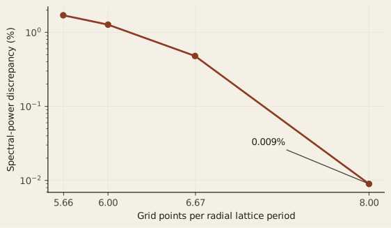
Download the frozen resolution data
| Points per period | \(\Delta x\) | Power discrepancy | Peak-density discrepancy |
|---|---|---|---|
| 5.66, shipped | 1.1107 | 1.70% | 1.07% |
| 6.00 | 1.0472 | 1.27% | 1.04% |
| 6.67 | 0.9425 | 0.48% | 0.29% |
| 8.00 | 0.7854 | 0.009% | 0.018% |
At eight points per period the power discrepancy is roughly 190 times smaller than at the shipped spacing. This motivates the showcase grid. The selected lattice wavenumber changes by less than \(5\times10^{-4}\) relative throughout the comparison; its small nonmonotone variation is not a convergence trend. The table measures mask sensitivity, and should not be read as an absolute error bound on every observable.
Regression checks cover checkpoint/restart consistency and selected CPU checksums. They support implementation consistency, not experimental validation. The showcase also needs its own conservation and late-time checks; a grid choice alone does not establish trustworthiness.
Performance
The retained Tungsten HIP strong-scaling series fixes the global problem at \(1280^3\) cells on LUMI-G. One MPI rank runs per MI250X GCD; eight GCDs make a node. The measurements cover 25 steps.
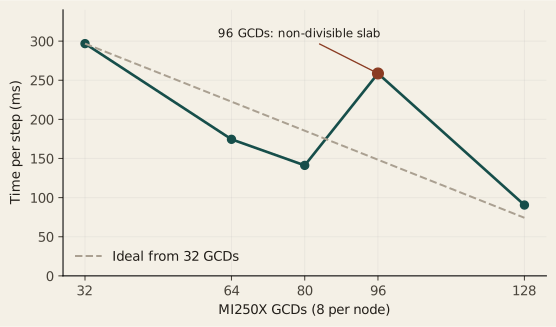
Download the frozen timing data
| GCDs | Nodes | Milliseconds / step |
|---|---|---|
| 32 | 4 | 296.83 |
| 64 | 8 | 174.51 |
| 80 | 10 | 141.19 |
| 96 | 12 | 258.67 |
| 128 | 16 | 90.49 |
The 96-GCD case is slower than the 64-GCD case despite using more hardware. Its slab count does not divide 1280. The data show that the process count and decomposition are part of the numerical execution design; adding ranks is not sufficient. The series supports this workload and machine, not a universal GPU scaling claim. Across the divisible endpoints, step time falls by a factor of 3.28 for four times the GCD count.
What the application does and does not do
What it does
- BCC density-field PFC and three-dimensional solidification.
- Single seeds, seed grids, and polycrystalline initial conditions.
- Conserved spectral ETD evolution in a periodic grid.
- CPU, CUDA, and HIP variants where their backends are configured.
- MPI and distributed FFTs through HeFFTe.
- Field output and checkpoint/restart.
- Grain-boundary and defect structures in the evolving density field.
- Front tracking and a moving density reservoir.
- An optional prescribed thermal drive.
What it does not do
- Track individual atoms as molecular dynamics does.
- Solve a physical free surface or real container walls.
- Solve heat transport or predict a melt pool from the prescribed drive.
- Model plasma exposure, irradiation damage, or fracture.
- Represent the separate TungstenLab research line.
- Establish general experimental validation from these calculations.
The published parameterization provides context; present repository-level calibration traceability is incomplete. The article reports model behavior and numerical evidence within that boundary.