Waves / Following a characteristic
A wave changes speed
A spatially varying coefficient turns a translating packet into a lesson about characteristics, resolution and time integration.
Download runnable lesson (.zip)
Includes the model, inputs, required headers and a short run guide.
The heat lessons smooth a field. Transport moves its values along characteristics instead. Program 6 of Trefethen (2000) uses Fourier differentiation and leapfrog for the periodic problem
\[ \begin{gathered} u_t+c(x)u_x=0, \\ c(x)=0.2+\sin^2(x-1), \\ u(x,0)=e^{-100(x-1)^2}, \\ 0\le x<2\pi. \end{gathered} \tag{1}\]
We reproduce that equation and add an exact characteristic reference. The Gaussian is periodically extended. Its endpoint mismatch is below \(4\times10^{-44}\), but it is not literally an analytic periodic Gaussian. The alternative cosine input is exactly periodic and useful for order checks.
Values travel; speeds vary
Along \(x'(t)=c(x(t))\), the chain rule gives \(d u(x(t),t)/dt=0\). The value is constant along the trajectory even while the packet stretches or compresses in physical coordinates. This is the nonconservative transport equation. Replacing \(c u_x\) with \((cu)_x\) would add \(c' u\) and define a different physical problem.
For \(a=0.2\), introduce a phase
\[ \begin{gathered} \phi(x)=\operatorname{atan2}\!\left(\sqrt{a+1}\sin(x-1), \sqrt a\cos(x-1)\right), \\ \phi'(x)=\frac{\sqrt{a(a+1)}}{c(x)}. \end{gathered} \tag{2}\]
Consequently \(\phi(x(t))\) increases at the constant rate \(\omega=\sqrt{a(a+1)}\). Subtracting \(\omega t\), inverting the angular map and wrapping the result into the interval gives the characteristic foot \(x_0\). The exact solution is \(u(x,t)=u(x_0,0)\):
double exact(double x, double t) const {
  if (!variable) {
    double foot = std::fmod(x - t, two_pi);
    if (foot < 0) foot += two_pi;
    return initial(foot);
  }
  constexpr double a = 0.2;
  const double phase = std::atan2(std::sqrt(a + 1) * std::sin(x - 1),
                                  std::sqrt(a) * std::cos(x - 1));
  const double foot_phase = phase - std::sqrt(a * (a + 1)) * t;
  double foot = 1 + std::atan2(std::sqrt(a) * std::sin(foot_phase),
                               std::sqrt(a + 1) * std::cos(foot_phase));
  if (foot < 0) foot += two_pi;
  return initial(foot);
}
The phase identity supplies a reference independently of the spectral derivative and the numerical time integrator.
A two-level method needs two states
Leapfrog approximates Equation 1 by
\[ u^{n+1}=u^{n-1}-2\Delta t\,c D_Nu^n. \tag{3}\]
There are two time sequences to initialize. The default constructs an approximate state at \(-\Delta t\) from a second-order Taylor expansion:
\[ u(-\Delta t)=f+\Delta t\,cf' +\tfrac12\Delta t^2c(c'f'+cf''). \tag{4}\]
The executable also offers the book’s startup expression. It uses the Gaussian shifted by \(0.2h/4\), as initialized before the book adjusts its timestep to the plotting interval. That expression does not equal the consistent negative-time Taylor state in Equation 4. Keeping both options visible lets us inspect the computational mode of a two-level scheme.
u.for_each_owned([&](int i, int j, int k) {
  const double x = u.coords(i, j, k)[0], c = model.speed(x);
  previous[u.idx(i, j, k)] =
      startup == "book" ? model.initial(x - 0.2 * two_pi / (4 * n))
                        : model.initial(x) + dt * c * model.first(x) +
                              0.5 * dt * dt * c *
                                  (model.speed_derivative(x) * model.first(x) +
                                   c * model.second(x));
});
Keep the spatial and temporal choices visible
for (int step = 1; step <= steps; ++step) {
  derivative.prepare();
  u.for_each_owned([&](int i, int j, int k) {
    const double x = u.coords(i, j, k)[0];
    next[u.idx(i, j, k)] = previous[u.idx(i, j, k)] -
                           2 * dt * model.speed(x) * derivative(i, j, k).x;
  });
  previous = u.vec();
  std::copy(next.begin(), next.end(), u.vec().begin());
  observe(step);
}
OpenPFC supplies the field, decomposition, FFT and requested x derivative. The leapfrog update and variable coefficient remain ordinary C++. All next values are computed before changing the current field. Copying into its existing buffer also preserves the evaluator’s storage binding.
For an even Fourier grid, a conservative leapfrog restriction is \(\Delta t\,c_{\max}N/2<1\). The executable rejects parameters that violate it. Stability alone does not guarantee that a narrow Gaussian is resolved or that the startup has suppressed the second temporal branch.
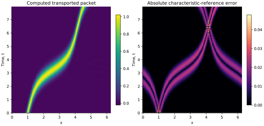
Run a short lesson or the book setup
openpfc run model.cpp input.json --launcher=none
openpfc run model.cpp trefethen-p6.json --launcher=none
The default uses the Taylor startup and ends at \(t=0.5\). The book preset uses \(N=128\), the book startup, \(\Delta t=0.0125\), and 636 steps ending at \(t=7.95\). Our periodic nodes begin at zero rather than \(h\); the sample ordering is cyclic, with the Gaussian’s tiny seam difference described above. These are mathematical reproductions and comparisons, not a bitwise MATLAB port.
Each attempt writes time slices and the characteristic reference in results/transport_rank_<rank>.csv. Try "initial": "cosine" and compare two timesteps at the same final time. The test checks second-order convergence for both constant and variable speed. Its independent Python reference traces characteristics with a small-step RK4 ODE integration, without using the C++ angular transformation.
Then compare the two startups with the Gaussian. Inspect successive steps as well as a distant final frame: a two-step oscillation can hide in an attractive space-time plot. For the continuous equation the weighted integral \(\int u/c\,dx\) is conserved, whereas \(\int u\,dx\) generally is not.
Continue with stability regions.
The complete C++ model and starting input are available with this lesson. Use the program 6 preset for the book’s Gaussian experiment.