Time integration / Stability geometry
Where a timestep is allowed to live
A stable PDE mode becomes an unstable computation if its scaled eigenvalue lands in the wrong part of the complex plane.
Download runnable lesson (.zip)
Includes the model, inputs, required headers and a short run guide.
The heat and transport examples have different timestep restrictions. To understand why, examine the scalar test equation \(y'=\lambda y\) and write \(z=\Delta t\lambda\). A one-step method maps \(y^n\) to \(R(z)y^n\). Its absolute-stability region is \(|R(z)|\le1\).
Program 25 of Trefethen (2000) compares the boundaries of Runge–Kutta, Adams–Bashforth, Adams–Moulton and backward-differentiation formulas. This example reproduces those families. The explicit RK tableaus are actual OpenPFC objects; the multistep formulas are example-local mathematical references, not newly supported library steppers.
Read stability from the tableau
For an explicit RK tableau, applying its stages to \(y'=\lambda y\) with \(y^n=1\) gives
\[ \begin{gathered} Y_i=1+z\sum_{j<i}a_{ij}Y_j, \\ R(z)=1+z\sum_i b_iY_i. \end{gathered} \tag{1}\]
The implementation follows those equations directly:
Complex amplification(const Tableau &method, Complex z) {
  std::vector<Complex> stage(method.stage_count(), 1);
  Complex result = 1;
  for (unsigned i = 0; i < method.stage_count(); ++i) {
    for (unsigned j = 0; j < i; ++j) stage[i] += z * method.a(i, j) * stage[j];
    result += z * method.b(i) * stage[i];
  }
  return result;
}
We use Euler, the midpoint rule, Kutta RK3 and classical RK4. Their stability polynomials are the first one, two, three and four terms beyond one in the exponential series. That identity provides an independent check of the tableau calculation; it is not how the program computes \(R\).
Different spectra ask different questions
Diffusion contributes negative real eigenvalues. Euler therefore requires \(-2\le\Delta t\lambda\le0\). Pure periodic advection contributes imaginary eigenvalues. Euler amplifies every nonzero imaginary mode since \(|1+i\eta|^2=1+\eta^2\). A smaller timestep reduces that amplification but does not create an imaginary-axis stability interval.
Higher-order RK methods have different regions. In particular, classical RK4 includes an interval on the imaginary axis. Higher order alone is not a license to choose a timestep without considering the operator’s spectrum.
for (int iy = 0; iy <= 140; ++iy) {
  for (int ix = 0; ix <= 140; ++ix) {
    const Complex z{-5 + ix * 0.05, -3.5 + iy * 0.05};
    grid << z.real() << ',' << z.imag();
    for (const auto &method : methods)
      grid << ',' << std::abs(amplification(method, z));
    grid << '\n';
  }
}
A root-locus picture for multistep formulas
For a recurrence with characteristic equation \(\rho(w)-z\sigma(w)=0\), a root on the unit circle gives the root-locus map \(z=\rho(e^{i\theta})/\sigma(e^{i\theta})\).
The Adams weights are obtained by integrating Lagrange interpolation polynomials through the method’s time nodes. The program independently checks their polynomial integration moments. Backward differentiation uses the backward-difference derivative series:
\[ \begin{gathered} z=\sum_{j=1}^{p}\frac{(1-w^{-1})^j}{j}, \\ |w|=1. \end{gathered} \tag{2}\]
for (int point = 0; point <= 400; ++point) {
  const double theta = 2 * std::numbers::pi * point / 400;
  const Complex w = std::polar(1.0, theta);
  Complex z = 0;
  if (ab || am) {
    Complex sigma = 0;
    for (std::size_t j = 0; j < nodes.size(); ++j)
      sigma += weights[j] * std::pow(w, nodes[j]);
    if (std::abs(sigma) < 1e-12)
      continue; // A pole is not a finite boundary point.
    z = (w - Complex{1}) / sigma;
  } else {
    const Complex difference = Complex{1} - Complex{1} / w;
    for (int j = 1; j <= order; ++j) z += std::pow(difference, j) / double(j);
  }
  boundary << family << ',' << order << ',' << theta << ',' << z.real() << ','
           << z.imag() << '\n';
}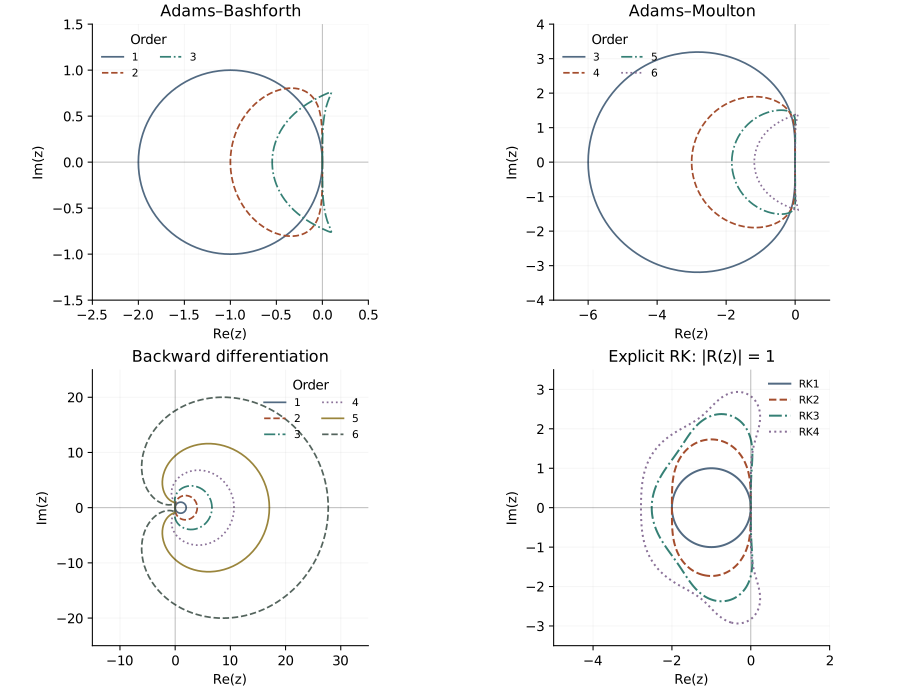
For a multistep method all roots must satisfy its root condition, with unit roots simple. A unit-root curve by itself is not permission to shade every enclosed region as stable. BDF1, for example, is stable outside its circle, including the negative real half-plane.
Experiment with a method rather than a label
openpfc run model.cpp input.json --launcher=noneThe empty input leaves the tableaus and plotting domain explicit in model.cpp. The output contains results/rk.csv with sampled stability-function magnitudes, and results/multistep.csv with root-locus points. Render them with the documented plotting script.
Predict the Euler and midpoint amplification at \(z=-2\) and at \(z=2i\). Then change the RK2 tableau from midpoint to Heun. Their internal stages differ, but their scalar stability polynomial should be identical. That does not make the methods identical on a nonlinear problem.
The test compares the computed RK magnitudes against independent Taylor polynomials and selected multistep negative/positive real intercepts. The diagram establishes properties of these formulas on the scalar test equation. Nonnormal operators, nonlinear dynamics and accuracy require additional analysis.
The complete C++ model and starting input are available with this lesson.