OpenPFC / Build a simulation
Compare one step with two half steps
Build adaptive exponential evolution from a linear Fourier symbol, a cubic reaction and explicit rollback.
Download runnable lesson (.zip)
Includes the model, inputs, required headers and a short run guide.
An exponential step treats a chosen linear operator exactly, but a nonlinear forcing still introduces time error. We refactor the adaptive ETD example into three tests of \(u_t=\Delta u-cu^3\) on a periodic domain: a pure heat mode (\(c=0\)), a spatially uniform cubic decay (\(c=1\)), and a nonuniform reaction–diffusion field. The same driver handles all three.
Make the split visible
struct ReactionDiffusion {
  pfc::Domain domain;
  pfc::Box3i box;
  double cubic;
  struct Local {
    double cubic;
    double nonlinearity(const pfc::sim::SpectralCell &cell) const {
      return -cubic * cell.psi * cell.psi * cell.psi;
    }
  };
  void declare_fields(pfc::SimulationState &state) const {
    pfc::sim::add_declared_field<double>(state, "psi", domain, box, 0);
  }
  double linear_symbol(double laplacian) const { return laplacian; }
  Local pointwise() const { return {cubic}; }
};
The library supplies the physical Laplacian symbol \(-\lVert k\rVert^2\); the model returns it unchanged. The local nonlinearity is \(-cu^3\). For a Fourier mode, the ETD1 update has the form
\[ \begin{gathered} \widehat u^*=e^{hL}\widehat u+h\varphi_1(hL)\widehat{N(u)}, \\ \varphi_1(z)=\frac{e^z-1}{z}, \\ \varphi_1(0)=1. \end{gathered} \tag{1}\]
The native implementation evaluates the small-argument limit robustly. The method’s linear exactness does not make its nonlinear part exact. See Cox and Matthews (2002) for the exponential-integration construction.
Estimate the error and preserve the accepted state
One full step produces \(u_h\); two half steps produce \(u_{h/2,h/2}\). Their difference is \(O(h^2)\) for this first-order method, so the controller uses error_order=2. On acceptance it keeps the two-half-step result; it does not Richardson-extrapolate it.
while (!time.done()) {
  if (++count > 10000) throw std::runtime_error("Attempt limit reached");
  const double t0 = time.get_accepted_time();
  time.begin_attempt(time.get_dt());
  const double dt = time.get_attempted_dt();
  doubling.attempt(t0, dt);
  const auto decision = controller.decide_from_embedded_error(
      dt, doubling.raw_difference(), doubling.saved_state(),
      doubling.half_steps(), comm);
  double rollback = 0;
  if (decision.accepted) {
    doubling.commit();
  } else {
    doubling.reject();
    for (std::size_t i = 0; i < u.vec().size(); ++i)
      rollback =
          std::max(rollback, std::abs(u.vec()[i] - doubling.saved_state()[i]));
  }
  controller.apply(time, decision);
Unlike the isolated candidate of the embedded RK lesson, this adapter leaves its trial field visible during an attempt. Rejecting must restore both the real field and its Fourier state. The model records the real-field rollback error for every rejected attempt. The library owns Fourier rollback and rebuilds the macro-step coefficients after commit or reject.
Check more than a controller metric
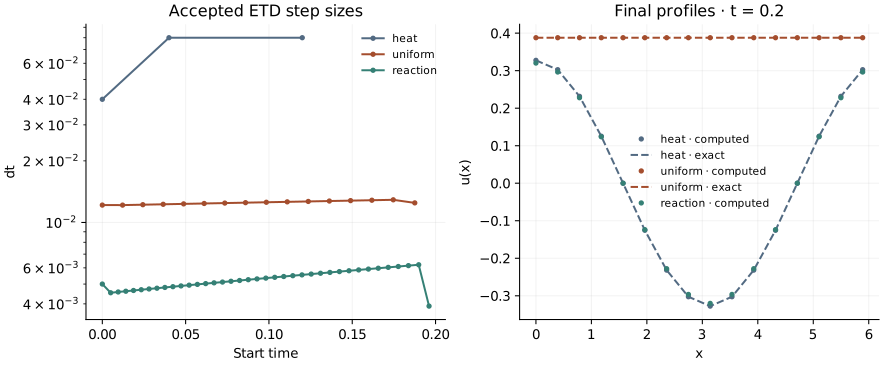
openpfc run model.cpp input.json --source-root .. --launcher=noneThe inputs choose even n, tolerance, initial dt and final end. The actual MPI size determines the decomposition; use --ranks=2 --launcher=mpirun to exercise distributed transforms. The grid is \(N\times4\times4\), with variation in x only. All lengths and wave numbers are physical.
For the heat case, \(u=.4e^{-t}\cos x\). For uniform reaction, \(u=.4/\sqrt{1+2(.4)^2t}\). The latter is not a heat eigenmode: its Laplacian vanishes and it tests the nonlinear time approximation alone. The nonuniform case is checked against an independent direct-DFT/RK4 reference on the same finite grid, not just another ETD run. Cubic products are sampled on the grid; no dealiasing study is claimed here.
Each rank writes an attempt ledger and the complete final fields. Checks also require unchanged rejected states and the documented plain-attempt work counts: three nonlinear evaluations and nine transforms. Adaptive error control is a time-accuracy decision, not a performance measurement.
The complete C++ model and starting input are available with this lesson. It also uses the shared lesson.hpp; keep its relative location when saving the files.