OpenPFC / Operators and their solutions
An asymmetric potential reshapes a membrane mode
Build a tensor-product eigenproblem with a steep potential and inspect its four lowest modes.
Download runnable lesson (.zip)
Includes the model, inputs, required headers and a short run guide.
A two-dimensional eigenfunction has geometry as well as an eigenvalue. Program 23 of Trefethen (2000) adds a steep nonnegative potential to the Dirichlet Laplacian on \([-1,1]^2\):
\[-\Delta u+e^{20(y-x-1)}u=\lambda u,\qquad u|_{\partial\Omega}=0.\]
The potential penalizes the region near the upper-left corner. The low modes should respond to this asymmetry; their contours are more informative than a table of numbers alone.
Combine one-dimensional operators in two directions
With x-fastest interior storage, apply \(-D^2\) along each row and column, then add the sampled potential to the diagonal.
for (int j = 0; j < m; ++j)
  for (int i = 0; i < m; ++i) {
    const int row = i + m * j;
    for (int k = 0; k < m; ++k) {
      a[row][k + m * j] -= d2[i + 1][k + 1];
      a[row][i + m * k] -= d2[j + 1][k + 1];
    }
    a[row][row] += std::exp(20 * (x[j + 1] - x[i + 1] - 1));
  }
const auto modes = eigen_reference::solve(eigen_reference::complex_matrix(a));
This example assembles the dense tensor matrix because the default degree 16 has only 225 interior unknowns. Its complex QR diagonalization is a bounded local reference, not a scalable OpenPFC eigenvalue solver. A large problem would require a suitable iterative eigensolver and operator action. The continuum operator is self-adjoint, but the raw Chebyshev collocation matrix is not Euclidean symmetric; we preserve that distinction.
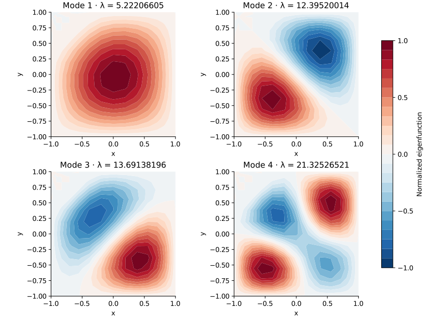
Read contours with the right invariances
openpfc run model.cpp input.json --source-root .. --launcher=noneresults/spectrum.csv records eigenvalues and scaled finite-matrix residuals; results/modes.csv records every point, including zero boundaries. Increase n from 12 to 16 before trusting a mode’s details. The steep potential can make matrix entries much larger than the low eigenvalues, so scaling matters when interpreting backward residuals.
An eigenvector’s sign is arbitrary. For clustered modes, even the basis inside a nearly degenerate eigenspace can change. Compare eigenvalues and subspaces rather than demanding one exact contour orientation. Independent checks reconstruct the operator and compare the low spectrum and residuals; they also verify all prescribed endpoint values. Continue with a forced Poisson problem using the same tensor idea.
The complete C++ model and starting input are available with this lesson. Keep collocation.hpp in the theme directory. This model also uses eigensystem.hpp in that directory.