OpenPFC / Operators and their solutions
Solve a square without a giant Kronecker matrix
Apply a Chebyshev tensor Laplacian through native GMRES, then check an exactly representable manufactured solution.
Download runnable lesson (.zip)
Includes the model, inputs, required headers and a short run guide.
Program 16 of Trefethen (2000) solves
\[ \begin{gathered} \Delta u=10\sin[8x(y-1)], \\ (x,y)\in[-1,1]^2, \\ u|_{\partial\Omega}=0. \end{gathered} \]
The textbook writes a Kronecker-sum matrix. We use the same degree-24 Chebyshev collocation equations and evaluate the tensor action directly inside OpenPFC GMRES. The physical model stays visible in its own file:
auto source = [=](double x, double y) {
  return manufactured ? -4 + 2 * x * x + 2 * y * y
                      : 10 * std::sin(8 * x * (y - 1));
};
auto boundary = [](double, double) { return 0.; };
return tensor::run(n, 0, source, boundary);
Apply each direction separately
For interior values \(U_{ij}\),
\[(\Delta_hU)_{ij}=\sum_k(D^2)_{ik}U_{kj}+\sum_k(D^2)_{jk}U_{ik}.\]
auto action = [&](const auto &v, auto &out) {
  std::fill(out.begin(), out.end(), 0);
  for (int j = 0; j < m; ++j)
    for (int i = 0; i < m; ++i) {
      const int row = i + m * j;
      out[row] = k2 * v[row];
      for (int k = 0; k < m; ++k)
        out[row] +=
            d2[i + 1][k + 1] * v[k + m * j] + d2[j + 1][k + 1] * v[i + m * k];
    }
};
The action uses \(O(N^3)\) arithmetic and \(O(N^2)\) field storage. It avoids forming the full \(O(N^4)\) tensor matrix. Full-restart GMRES still stores its Krylov basis, so this small reference does not claim a memory-optimal large-scale solver. The reference Chebyshev matrix is example-owned; GMRES and its true-residual admission are native OpenPFC capabilities.
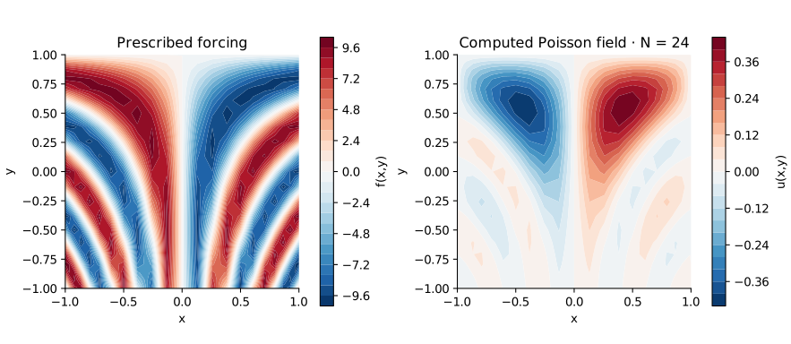
Manufacture a solution before changing the forcing
Set manufactured=true to use \(u=(1-x^2)(1-y^2)\) and \(f=-4+2x^2+2y^2\). Both boundary values vanish and the polynomial is exactly representable for degree at least two in each axis. Any remaining error comes from arithmetic and the linear solve, not an unresolved manufactured function.
openpfc run model.cpp input.json --source-root .. --launcher=noneThe attempt writes all nodes and values to results/solution.csv and prints the unpreconditioned equation residual. The checks verify the manufactured field, compare the original low-degree forcing problem with an independent Lagrange/dense solve, and separately inspect the book’s default resolution. A converged linear solver solves its discrete equations; the choice of resolution still controls how well they represent the PDE.
The complete C++ model and starting input are available with this lesson. Keep collocation.hpp in the theme directory. This model also uses tensor.hpp in that directory.