OpenPFC / Operators and their solutions
Let the boundary drive the interior
Eliminate prescribed edge values into the right-hand side and solve a homogeneous interior Laplace equation.
Download runnable lesson (.zip)
Includes the model, inputs, required headers and a short run guide.
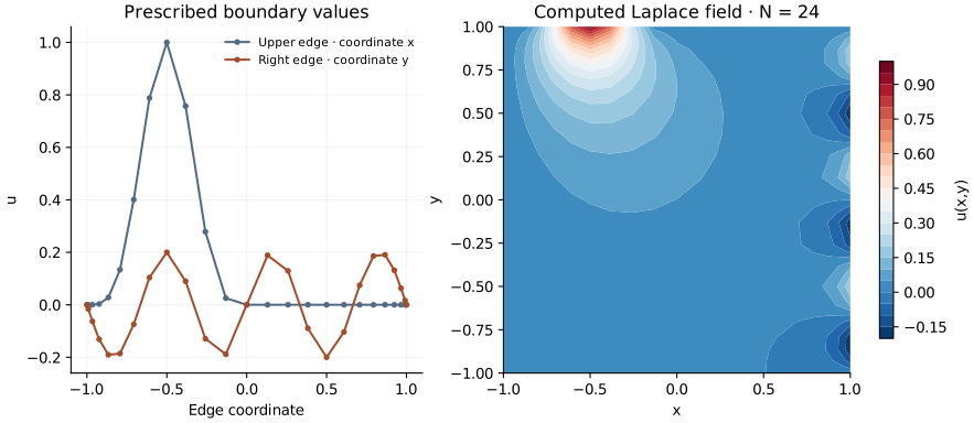
A zero interior forcing need not produce a zero field. Program 36 of Trefethen (2000) solves \(\Delta u=0\) on the square with nonzero prescribed edge data. The upper edge has \(\sin^4(\pi x)\) for \(x<0\); the right edge has \(.2\sin(3\pi y)\). Other edge values are zero.
auto source = [](double, double) { return 0.; };
auto boundary = [=](double x, double y) {
  if (manufactured) return x * x - y * y;
  return (y == 1 && x < 0 ? std::pow(std::sin(std::numbers::pi * x), 4) : 0) +
         (x == 1 ? .2 * std::sin(3 * std::numbers::pi * y) : 0);
};
return tensor::run(n, 0, source, boundary);
Move known endpoint contributions to the other side
For each interior equation, split the tensor sum into unknown interior values and known edge values. The latter enter the right-hand side with a minus sign. This gives the same collocation solution as retaining all nodes and replacing boundary rows by identity equations, as the book does. The shared solver keeps the known values in the output grid and solves only for interior unknowns with native GMRES.
This is prescribed-value elimination, not a periodic FFT trick. The one-dimensional boundary lesson derives the same distinction for homogeneous and lifted endpoint data.
Check a harmonic polynomial with all four edges active
openpfc run model.cpp input.json --source-root .. --launcher=noneSet manufactured=true to prescribe \(u=x^2-y^2\) on every edge. Its Laplacian is zero, giving an independent complete-field oracle for the elimination signs and boundary indexing. The normal input reproduces the book’s piecewise edge functions. Every node appears in results/solution.csv.
The checks verify both the exact manufactured field and a low-degree reference solve with the original edge values. The cutoff of the upper edge data at x=0 also limits regularity; increasing degree cannot make those prescribed data smoother. Assess convergence in the interior and near the boundary separately rather than interpreting a visually smooth plot as a uniform accuracy certificate.
The complete C++ model and starting input are available with this lesson. Keep collocation.hpp in the theme directory. This model also uses tensor.hpp in that directory.