Polynomial methods / Learn by experiment
A boundary condition changes an equation
Solve three Chebyshev Poisson problems with OpenPFC GMRES: homogeneous, lifted and mixed boundary data.
Download runnable lesson (.zip)
Includes the model, inputs, required headers and a short run guide.
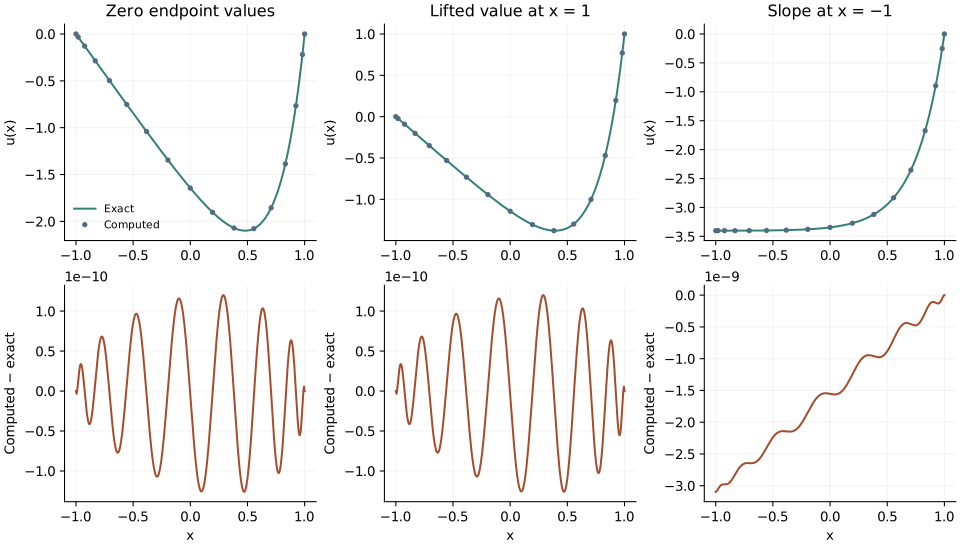
All three experiments solve \(u''=e^{4x}\) on \([-1,1]\). What changes is the information supplied at the endpoints. Programs 13, 32 and 33 of Trefethen (2000) show how zero values, a nonzero value, and a specified slope enter a collocation calculation.
Differentiate before removing boundary values
Form \(D^2\) on the complete grid, then select equations and unknowns. Squaring an already truncated first-derivative matrix would discard endpoint contributions and give a different second derivative. For \(u(-1)=u(1)=0\), retain only the interior block of \(D^2\).
For \(u(-1)=0\), \(u(1)=1\), write \(u=v+(x+1)/2\). The lift satisfies the boundary values and its second derivative is zero. The interior system for \(v\) is therefore the same homogeneous-boundary problem.
For \(u'(-1)=0\), \(u(1)=0\), retain the value at \(-1\) as an unknown and replace the equation there with the corresponding row of \(D\). The derivative row is evaluated at \(-1\), which is the last node in this storage order.
for (const std::string boundary : {"zero", "lifted", "mixed"}) {
  const bool mixed = boundary == "mixed";
  const int count = mixed ? n : n - 1;
  polynomial::Matrix a(count, polynomial::Vector(count));
  polynomial::Vector f(count);
  for (int row = 0; row < count; ++row) {
    const int i = row + 1;
    const auto &equation = mixed && i == n ? d[i] : d2[i];
    f[row] = mixed && i == n ? 0 : std::exp(4 * x[i]);
    for (int col = 0; col < count; ++col) a[row][col] = equation[col + 1];
  }
  const auto interior = polynomial::solve(a, f);
  polynomial::Vector u(n + 1);
  std::copy(interior.begin(), interior.end(), u.begin() + 1);
  if (boundary == "lifted")
    for (int j = 0; j <= n; ++j) u[j] += (x[j] + 1) / 2;
OpenPFC GMRES solves these example-owned collocation systems. They illustrate boundary equations; they do not advertise a public Chebyshev boundary operator or attach a nonperiodic boundary condition to a periodic FFT. The integration chapter explains row scaling and the native linear-solver contract.
Three answers that can be checked independently
For zero boundary values,
\[u_0(x)=\frac{e^{4x}-x\sinh4-\cosh4}{16}. \tag{1}\]
The lifted solution is \(u_0(x)+(x+1)/2\). For the mixed conditions,
\[u_m(x)=\frac{e^{4x}-4e^{-4}(x-1)-e^4}{16}. \tag{2}\]
Differentiate these formulas and substitute the endpoints before looking at a plot. This checks both the forcing and the boundary signs.
Experiment with the boundary, not only the resolution
openpfc run model.cpp input.json --source-root .. --launcher=noneresults/solutions.csv labels each case and distinguishes grid nodes from an interpolated curve. The default n=16 repeats the book’s degree. Try 8 and 24; compare the entire curve with the analytic solution. The tests check all three curves, both endpoint values where prescribed, and the Neumann equation using an independent Lagrange derivative at the endpoint.
As an exercise, lift arbitrary values \(u(-1)=a\), \(u(1)=b\) with \(\ell(x)=a(1-x)/2+b(1+x)/2\). Then change the slope condition to a nonzero value and modify its right-hand side. A derivative row is an equation, not a special flag whose meaning the linear solver can infer.
The complete C++ model and starting input are available with this lesson. It also uses the shared collocation.hpp; keep its relative location when saving the files.