Polynomial methods / Learn by experiment
Where should the samples go?
Compare equally spaced and Chebyshev nodes without changing the function or polynomial degree.
Download runnable lesson (.zip)
Includes the model, inputs, required headers and a short run guide.
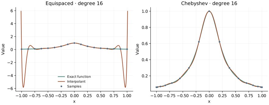
A polynomial can pass through every sample and still be a poor approximation between them. Program 9 of Trefethen (2000) makes that distinction visible with \(f(x)=1/(1+16x^2)\) and degree \(N=16\). We use the same experiment, replacing monomial fitting with barycentric evaluation (Berrut and Trefethen 2004).
Change the nodes, keep the question
An equally spaced grid has \(x_j=-1+2j/N\). A Chebyshev grid projects equally spaced angles onto the interval:
\[ \begin{gathered} x_j=\cos(j\pi/N), \\ j=0,\ldots,N. \end{gathered} \tag{1}\]
Both grids contain \(N+1\) values. Both determine a unique polynomial of degree at most \(N\). The Chebyshev points cluster near the endpoints, where the uniform-grid interpolant has its largest oscillations.
inline Vector nodes(int n, bool chebyshev = true) {
  Vector x(n + 1);
  for (int j = 0; j <= n; ++j)
    x[j] = chebyshev ? std::cos(std::numbers::pi * j / n) : -1.0 + 2.0 * j / n;
  return x;
}
Evaluate a polynomial without fitting its monomials
For distinct nodes, define \(w_j=1/\prod_{k\ne j}(x_j-x_k)\). The barycentric formula is
\[p(x)=\frac{\sum_j w_jf_j/(x-x_j)}{\sum_j w_j/(x-x_j)}. \tag{2}\]
At a node we return the corresponding sample directly; evaluating the fraction there would divide by zero. Multiplying every weight by the same nonzero constant leaves the interpolant unchanged. The example uses the general product formula at these small degrees; specialised Chebyshev weights and more careful weight construction are preferable at large sizes.
class Interpolant {
  Vector x_, values_, weights_;

public:
  Interpolant(Vector x, Vector values)
      : x_(std::move(x)), values_(std::move(values)), weights_(x_.size(), 1) {
    if (values_.size() != x_.size())
      throw std::invalid_argument("Sample sizes differ");
    for (std::size_t j = 0; j < x_.size(); ++j)
      for (std::size_t k = 0; k < x_.size(); ++k)
        if (j != k) weights_[j] /= x_[j] - x_[k];
  }
  double operator()(double point) const {
    double numerator = 0, denominator = 0;
    for (std::size_t j = 0; j < x_.size(); ++j) {
      if (point == x_[j]) return values_[j];
      const double term = weights_[j] / (point - x_[j]);
      numerator += term * values_[j];
      denominator += term;
    }
    return numerator / denominator;
  }
};
The interpolant is example-owned mathematics. This introductory chapter supplies the evaluator used by the subsequent OpenPFC solver experiments; it does not imply that OpenPFC provides a public polynomial-interpolation API.
for (bool chebyshev : {false, true}) {
  const auto x = polynomial::nodes(n, chebyshev);
  polynomial::Vector values;
  for (double point : x) values.push_back(1 / (1 + 16 * point * point));
  const polynomial::Interpolant interpolate(x, values);
  const auto name = chebyshev ? "chebyshev" : "equispaced";
  for (int j = 0; j <= n; ++j)
    output << name << ",node," << x[j] << ',' << values[j] << ',' << values[j]
           << '\n';
  for (int j = 0; j <= 404; ++j) {
    const double point = -1.01 + .005 * j;
    output << name << ",curve," << point << ',' << interpolate(point) << ','
           << 1 / (1 + 16 * point * point) << '\n';
  }
}
Make the oscillations visible
openpfc run model.cpp input.json --source-root .. --launcher=noneThe CSV results/interpolation.csv distinguishes node and curve records. The curve follows the book’s range \([-1.01,1.01]\): the outermost \(0.01\) at each end is extrapolation. Assess interpolation errors on \([-1,1]\) separately. Change n from 16 to 24 and predict which grid will improve. Increasing the degree on equally spaced points does not guarantee convergence; barycentric evaluation cannot repair an ill-conditioned approximation problem.
The regression check compares the complete default curve with an independent Lagrange-basis evaluation and checks every node. Continue with the nodal polynomial to see the node geometry in the complex plane.
The complete C++ model and starting input are available with this lesson. It also uses the shared collocation.hpp; keep its relative location when saving the files.