Polynomial methods / Learn by experiment
The geometry behind an interpolation error
See how the product of distances to the nodes shapes polynomial approximation on the real and complex planes.
Download runnable lesson (.zip)
Includes the model, inputs, required headers and a short run guide.
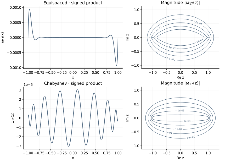
Why did changing the nodes help the previous interpolant? Program 10 of Trefethen (2000) looks at the polynomial that vanishes at all those nodes:
\[\omega_{N+1}(z)=\prod_{j=0}^{N}(z-x_j). \tag{1}\]
This is a monic polynomial of degree \(N+1\), not the degree-\(N\) interpolant of the previous chapter. The distinction is useful: one describes the node geometry, while the other also depends on the sampled values.
Multiply distances directly
For a real argument we draw the signed product; for a complex argument we draw its magnitude. C++’s std::complex<double> makes the same expression work for both. Forming monomial coefficients first is unnecessary.
for (bool chebyshev : {false, true}) {
  const auto nodes = polynomial::nodes(n, chebyshev);
  auto product = [&](std::complex<double> z) {
    std::complex<double> value = 1;
    for (double x : nodes) value *= z - x;
    return value;
  };
  const auto name = chebyshev ? "chebyshev" : "equispaced";
  for (int i = 0; i <= 400; ++i) {
    const double x = -1 + .005 * i;
    line << name << ',' << x << ',' << product(x).real() << '\n';
  }
  for (int j = 0; j <= 112; ++j)
    for (int i = 0; i <= 140; ++i) {
      const double x = -1.4 + .02 * i, y = -1.12 + .02 * j;
      plane << name << ',' << x << ',' << y << ',' << std::abs(product({x, y}))
            << '\n';
    }
}
This chapter is a mathematical reference implemented with the C++ standard library and the collection’s small example-local node helper. The following chapters connect these nodes to OpenPFC’s FFT and linear solvers.
Read the error formula carefully
For a sufficiently differentiable real function and a real interpolation point, the classical remainder has the form
\[f(x)-p_N(x)=\frac{f^{(N+1)}(\xi_x)}{(N+1)!}\omega_{N+1}(x). \tag{2}\]
A small nodal product helps, but the derivative factor also matters. For analytic functions, nearby complex singularities influence approximation. Contours of \(|\omega(z)|\) illustrate this geometry; they are not contours of the actual interpolation error for an arbitrary function.
Try another degree
openpfc run model.cpp input.json --source-root .. --launcher=noneresults/nodal.csv holds the real curves. results/potential.csv holds the complex-plane magnitudes on the book’s rectangular grid. Change n to 8 or 24 and keep the contour levels fixed before comparing. Auto-scaling each plot independently can conceal the very difference we want to see.
For Chebyshev extrema nodes there is an independent identity,
\[\omega_{N+1}(z)=2^{1-N}(z^2-1)U_{N-1}(z),\]
where \(U_0=1\), \(U_1=2z\), and \(U_{k+1}=2zU_k-U_{k-1}\). The regression check uses this recurrence to verify the complex-plane product, including its scale. This is a numerical identity check, not a proof of the remainder theorem or a guarantee about every function one might interpolate.
The complete C++ model and starting input are available with this lesson. It also uses the shared collocation.hpp; keep its relative location when saving the files.