OpenPFC / Operators and their solutions
A wave number can make a solve delicate
Keep the tensor discretization and add a Helmholtz shift that changes the spectrum and conditioning.
Download runnable lesson (.zip)
Includes the model, inputs, required headers and a short run guide.
Keep the square, zero endpoint values and polynomial grid, but solve
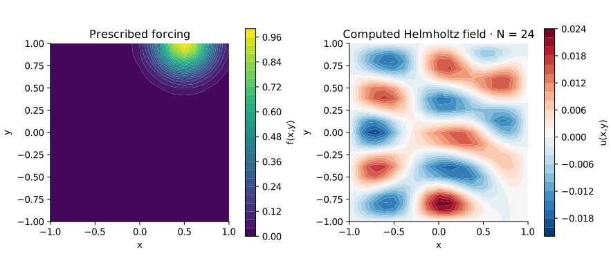
\[\Delta u+k^2u=e^{-10[(y-1)^2+(x-.5)^2]}.\]
Program 17 of Trefethen (2000) chooses \(k=9\). The source is concentrated near the top boundary, while the solution can oscillate throughout the interior. This is an elliptic boundary solve, not a time-marching wave.
auto source = [=](double x, double y) {
  return manufactured
             ? -4 + 2 * x * x + 2 * y * y +
                   wave * wave * (1 - x * x) * (1 - y * y)
             : std::exp(-10 * ((y - 1) * (y - 1) + (x - .5) * (x - .5)));
};
auto boundary = [](double, double) { return 0.; };
return tensor::run(n, wave * wave, source, boundary);
A diagonal shift changes the solver’s assumptions
The shared tensor action adds \(k^2U_{ij}\) to the Laplacian action. Even though \(-\Delta\) with homogeneous Dirichlet values is positive definite, \(\Delta+k^2I\) can be indefinite or singular. We therefore use native GMRES, not a method that assumes positive definiteness. Its diagonal inverse is only a preconditioner; it does not decide the physical boundary condition.
auto action = [&](const auto &v, auto &out) {
  std::fill(out.begin(), out.end(), 0);
  for (int j = 0; j < m; ++j)
    for (int i = 0; i < m; ++i) {
      const int row = i + m * j;
      out[row] = k2 * v[row];
      for (int k = 0; k < m; ++k)
        out[row] +=
            d2[i + 1][k + 1] * v[k + m * j] + d2[j + 1][k + 1] * v[i + m * k];
    }
};
Continuum resonances satisfy \(k^2=(\pi^2/4)(m^2+n^2)\) for positive integers m,n. Near one of them, a small change in forcing or resolution can change the amplitude strongly. At a resonance an arbitrary forcing need not admit a unique solution.
Give the shifted problem its own oracle
openpfc run model.cpp input.json --source-root .. --launcher=noneThe inputs are n, wave and manufactured. The manufactured mode uses \(u=(1-x^2)(1-y^2)\), with its matching \(\Delta u+k^2u\) on the right-hand side. All final nodes are in results/solution.csv. The checks compare that field with its exact formula and the book forcing with an independent small dense system. A separate reference inspects the default degree 24.
Try changing wave before changing n. Distinguish a genuine near-resonant amplitude from a failure to resolve the spatial solution. More GMRES iterations cannot fix either an inappropriate boundary condition or the absence of a unique continuum solution. Compare next with nonzero boundary data.
The complete C++ model and starting input are available with this lesson. Keep collocation.hpp in the theme directory. This model also uses tensor.hpp in that directory.