OpenPFC / A conserved nonlinear model
Let a conserved field separate into phases
Separate the local free-energy derivative from the differential operators. Three short functions then state the physics.
Download runnable lesson (.zip)
Includes the model, inputs, required headers and a short run guide.
A diffuse interface balances a local preference for two phases against a gradient penalty, following the free-energy construction of Cahn and Hilliard (1958). For a periodic square, take
\[ \begin{aligned} F[c]&=\int_\Omega f(c,\nabla c)\,d\mathbf x,\\ f(c,\nabla c)&=\frac{(c^2-1)^2}{4}+\frac\gamma2|\nabla c|^2,\\ \mu&=c^3-c-\gamma\Delta c,\\ c_t&=M\Delta\mu. \end{aligned} \tag{1}\]
Unlike Allen–Cahn, this kinetic law conserves the mean composition. For a smooth periodic continuum solution, integration by parts gives \(dF/dt=-M\int|\nabla\mu|^2\,d\mathbf x\le0\).
Put the linear and nonlinear pieces in their own places
For a Laplacian symbol \(\ell=-|\mathbf k|^2\), write \(L=-M\ell(1+\gamma\ell)\) and \(\widehat{\mathcal N}=M\ell\,\widehat{c^3}\).
struct CahnHilliard {
  pfc::Domain domain;
  pfc::Box3i box;
  double mobility, gamma, cubic;

  void declare_fields(pfc::SimulationState &state) const {
    pfc::sim::add_declared_field<double>(state, "psi", domain, box, 0);
  }
  double linear_symbol(double laplacian) const {
    return -mobility * laplacian * (1 + gamma * laplacian);
  }
  double nonlinear_symbol(double laplacian) const { return mobility * laplacian; }
  struct Local {
    double cubic;
    double nonlinearity(const pfc::sim::SpectralCell &cell) const {
      return cubic * cell.psi * cell.psi * cell.psi;
    }
  };
  Local pointwise() const { return {cubic}; }
};
The local callable evaluates only the cubic. nonlinear_symbol applies its Laplacian in Fourier space. The field declaration tells the system where the primary psi state lives. No model-specific time loop or FFT bookkeeping belongs inside those three formulas.
Use the native spectral ETD system
pfc::SimulationState state;
physics.declare_fields(state);
auto &u = state.get_field<double>("psi");
u.apply([&](double x, double y, double) {
  const double a = 2 * std::numbers::pi * x / length;
  const double b = 2 * std::numbers::pi * y / length;
  return mean +
         (initial == "constant"
              ? 0
              : amplitude * (initial == "mode" ? std::cos(a) * std::cos(b)
                                               : std::cos(a) + std::sin(2 * b) +
                                                     std::cos(2 * a + b)));
});
pfc::sim::SpectralETDSystem system(physics, stack.fft(), state, dt);
The initial mixture is a deterministic sum of physical Fourier modes. It therefore has the same values at a given global sample on every MPI partition. This replaces the older example’s rank-local random stream and makes cross-rank comparisons meaningful.
for (int step = 1; step <= steps; ++step) {
  system.step((step - 1) * dt);
  if (step % save_every == 0 || step == steps) observe(step);
}
ETD1 advances
\[ \begin{aligned} \hat c^{m+1}&=e^{L\Delta t}\hat c^m\\ &\quad+\Delta t\,\varphi_1(L\Delta t)\widehat{\mathcal N(c^m)}. \end{aligned} \tag{2}\]
The native coefficient calculation uses the limiting value \(\varphi_1(0)=1\) and stable evaluation near zero; it does not discard the nonlinear contribution whenever \(L=0\). Cox and Matthews (2002) explains exponential time differencing for stiff systems.
Check conservation separately from dissipation
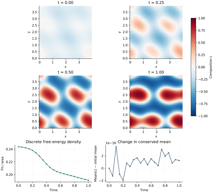
Both symbols vanish at zero wave number, so the mean is conserved to roundoff. The diagnostic energy uses the discrete Fourier Laplacian, \(\langle(c^2-1)^2/4+\gamma c(-\Delta_hc)/2\rangle\). The mean-angle brackets denote the grid average, so this is energy per unit area. It agrees with the discrete gradient-flow energy rather than assuming that sampled first derivatives retain every Nyquist mode.
This first-order explicit nonlinear treatment is not unconditionally energy stable. Its pointwise cubic is also not de-aliased. A decreasing curve for the displayed run is an observation, not a general guarantee. Refine both timestep and grid before interpreting an interface.
Run a model with an answer you already know
openpfc run model.cpp input.json --launcher=noneSet initial: "constant": every mode except the conserved mean vanishes. Set initial: "mode", mean: 0 and cubic: 0 to isolate the linear growth rate \(M|\mathbf k|^2(1-\gamma|\mathbf k|^2)\). The tests check these exact limits and compare complete nonlinear small-grid fields with an independent direct Fourier calculation on one and two ranks. With cubic: 0, the recorded potential becomes \(-c^2/2+1/4\), matching that intentionally modified linear model.
Two companion inputs refine one numerical choice at a time while keeping the physical end time at 1:
openpfc run model.cpp refine-grid.json --launcher=none
openpfc run model.cpp refine-time.json --launcher=none
Compare the degree-128 final field at every second node with the degree-64 result, then compare the two degree-64 timesteps. The grid refinement input and time refinement input save initial and final fields to keep the comparisons small.
In the checked CPU run, the maximum differences were about \(2\times10^{-11}\) for grid refinement and \(6.5\times10^{-4}\) for timestep refinement. These are comparisons between discrete solutions, not errors against an exact nonlinear PDE solution. For this configured case, changing the timestep has a much larger effect than refining the grid.
The default \(64^2\) grid, .001 timestep and deterministic initial field replace the old \(512^2\) random-field demo while preserving its PDE and ETD1 method. The new box length is 4 and \(\gamma=.04\), so an interface scale \(\sqrt{2\gamma}\approx.28\) spans about 4.5 grid intervals. These choices give a small demonstration with resolved interfaces; keeping the old length 20 and \(\gamma=.01\) on only 64 points would not. results/fields_rank_*.csv contains saved physical fields; rank zero writes mean and energy to results/diagnostics.csv. The complete source and input are available.