Interpolation / What the samples say
A curve hidden between the samples
Passing through every sample does not determine every feature of the curve between them.
Download runnable lesson (.zip)
Includes the model, inputs, required headers and a short run guide.
Program 3 of Trefethen (2000) reconstructs a discrete spike, a square pulse, and a hat from equally spaced samples. Their cardinal interpolants all pass through the supplied values. Their behaviour between those values can be much less obvious.
Build a cardinal basis
At spacing \(h=1\), define
\[ \operatorname{sinc}(s)=\begin{cases}1,&s=0,\\ \sin(\pi s)/(\pi s),&s\ne0, \end{cases} \qquad p(x)=\sum_{j=-10}^{10}u_j\operatorname{sinc}(x-j). \tag{1}\]
At an integer node \(m\), all basis functions except the \(m\)th vanish, so \(p(m)=u_m\). This is an interpolation property, not an error estimate for an unknown underlying physical field. The finite sum implicitly extends the discrete data by zero outside the stated node set.
double sinc(double x) {
  if (std::abs(x) < 1e-14) return 1;
  const double angle = std::numbers::pi * x;
  return std::sin(angle) / angle;
}

double interpolate(const pfc::data::Field<double> &samples, double x) {
  double value = 0;
  samples.for_each_owned([&](double node, double, double, double sample) {
    value += sample * sinc(x - node); // The sample spacing is h = 1.
  });
  return value;
}
OpenPFC supplies the field, coordinates and owned-cell iteration. The sinc reconstruction is example-local mathematics; it is not presented as a generic interpolation service in the library.
Ask three different questions of the same basis
The spike has one nonzero sample at zero. Its interpolant is one sinc. The square pulse has value one for \(|j|\le3\) and zero elsewhere. The hat has nodal values \(\max(0,1-|j|/3)\).
for (int profile = 0; profile < 3; ++profile) {
  samples.apply([&](double x, double, double) {
    if (profile == 0) return x == 0 ? 1.0 : 0.0;
    if (profile == 1) return std::abs(x) <= 3 ? 1.0 : 0.0;
    return std::max(0.0, 1 - std::abs(x) / 3);
  });
  for (int point = 0; point <= 400; ++point) {
    const double x = -10.0 + point / 20.0;
    output << profile << ',' << x << ',' << interpolate(samples, x) << '\n';
  }
  samples.for_each_owned([&](double x, double, double, double sample) {
    nodal_error =
        std::max(nodal_error, std::abs(interpolate(samples, x) - sample));
  });
}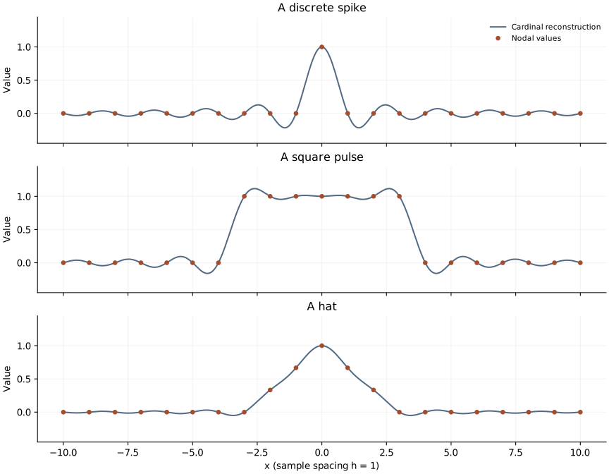
The square pulse overshoots between samples even though every sample is interpolated correctly. The continuous band-limited interpolant is not the original discontinuous step function. Hiding the oscillation by clipping the curve would change the reconstruction and conceal the lesson.
Run and look between the points
openpfc run model.cpp input.json --launcher=noneThis example runs on one process. The empty input leaves the node set and three profiles visible in model.cpp. The attempt directory’s results/interpolation.csv contains 401 evaluation points for each of the three profiles.
Check values at integer x coordinates first, then near the square pulse’s edge. The test checks every nodal value, the complete spike reconstruction against one analytic sinc, and the existence of a square-pulse overshoot. That combination checks both interpolation and a revealing consequence between nodes.
As an experiment, change the square pulse from seven nonzero samples to three. Predict what happens to the central plateau and edge oscillations. Then change the evaluation spacing without changing the input samples. The reconstructed function should stay the same: you have changed its display sampling, not the interpolation problem.
The domain is not a periodic Fourier grid
The sample field has nonperiodic metadata and includes both endpoints \(-10\) and \(10\). We do not wrap the sinc tails around this interval. Periodic trigonometric interpolation is a different basis and boundary assumption, developed in the matrix/FFT differentiation lesson.
The complete C++ model and starting input are available with this lesson.