Differentiation / Matrix or transform
One derivative, two algorithms
If a derivative rings near a corner, changing a matrix multiply into an FFT will not remove the corner.
Download runnable lesson (.zip)
Includes the model, inputs, required headers and a short run guide.
Programs 4 and 5 of Trefethen (2000) make a valuable comparison: calculate the same periodic spectral derivative with a dense matrix and with an FFT. The approximation is the trigonometric interpolant; the algorithms are two ways to differentiate it. We repeat both of the book’s profiles, a hat and \(e^{\sin x}\), with independent C++ code.
Differentiate the interpolating basis
For an even number \(N\) of points \(x_j=2\pi j/N\), the first-derivative matrix is
\[ D_{ij}=\begin{cases} 0,&i=j,\\ \tfrac12(-1)^{i-j}\cot\!\left(\tfrac{x_i-x_j}{2}\right),&i\ne j. \end{cases} \tag{1}\]
The zero diagonal and alternating off-diagonal terms encode a global periodic interpolant. They are not a high-order local stencil. The example-local implementation in ../profiles.hpp is small enough to read:
inline double matrix_derivative(std::span<const double> samples, int row) {
  const int n = static_cast<int>(samples.size());
  const double h = 2 * std::numbers::pi / n;
  double derivative = 0;
  for (int column = 0; column < n; ++column) {
    if (column == row) continue;
    const int difference = row - column;
    const double sign = difference % 2 == 0 ? 1.0 : -1.0;
    derivative += 0.5 * sign / std::tan(difference * h / 2) * samples[column];
  }
  return derivative;
}
The matrix action takes \(O(N^2)\) operations for all rows. The FFT route transforms the same samples, multiplies Fourier coefficients by \(ik\), and transforms back in \(O(N\log N)\) work. For real-valued data, the even-grid Nyquist first derivative is zero in both representations.
Compare actual values
for (const auto name : {"hat", "analytic"}) {
  std::vector<double> samples(n);
  for (int j = 0; j < n; ++j) samples[j] = profiles::evaluate(name, j * h).value;
  u.apply([&](double x, double, double) {
    return profiles::evaluate(name, x).value;
  });
  derivative.prepare();
  u.for_each_owned([&](int i, int j, int k) {
    const auto global = u.box().low;
    if (j + global[1] != 0 || k + global[2] != 0) return;
    const double x = (i + global[0]) * h;
    const auto exact = profiles::evaluate(name, x);
    const double dense = profiles::matrix_derivative(samples, i + global[0]);
    const double fourier = derivative(i, j, k).x;
    agreement = std::max(agreement, std::abs(dense - fourier));
    output << name << ',' << x << ',' << u(i, j, k) << ',' << dense << ','
           << fourier << ',' << exact.derivative << ',' << exact.differentiable
           << '\n';
  });
}
OpenPFC owns the sampled field, MPI decomposition, transforms, and spectral evaluator. The cotangent formula is a mathematical reference local to this example, not a newly advertised public dense-matrix API.
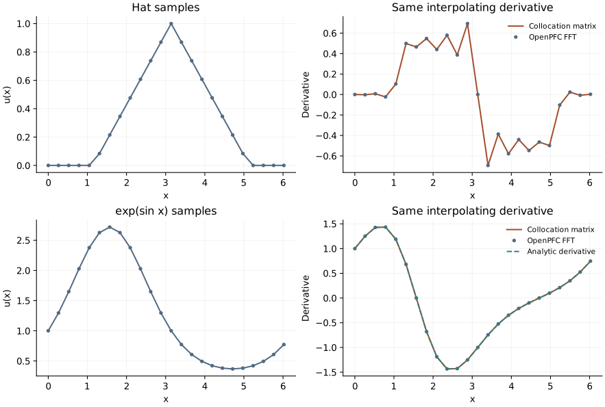
The hat is \(u(x)=\max(0,1-|x-\pi|/2)\). Its derivative is discontinuous at the peak and support edges. At those corners the classical derivative is undefined. The CSV marks such points with differentiable=0; it does not pretend that an arbitrary chosen slope is an exact derivative there.
For \(e^{\sin x}\) the independent exact derivative is \(\cos x\,e^{\sin x}\). At the default \(N=24\), the approximation is already very accurate. Matching algorithms alone would not establish that fact; the analytic reference does.
Run both experiments
openpfc run model.cpp input.json --source-root .. --launcher=noneThe input sets n. The shared-header source root preserves ../profiles.hpp. Each attempt writes results/derivative_rank_<rank>.csv for both profiles, with actual sample, matrix derivative, Fourier derivative, and exact reference where defined.
Double n. The analytic error should shrink toward roundoff, while the hat derivative retains oscillation near corners. Compare the curves at fixed physical distance from a corner and then within a few grid cells of it: those are different limits. Use two MPI ranks and verify the same global samples rather than assuming every rank owns the x-axis slice.
The ordinary checks compare matrix and FFT values, require the analytic derivative to agree within \(10^{-10}\), and validate the complete set of recorded samples. They do not claim uniform convergence at nondifferentiable points. Continue with what smoothness buys you.
The complete C++ model and starting input are available with this lesson. It also uses the shared profiles.hpp; keep its relative location when saving the files.