OpenPFC / Operators and their solutions
A periodic potential splits eigenvalues
Track the eleven lowest periodic Mathieu eigenvalues as the strength of a cosine potential changes.
Download runnable lesson (.zip)
Includes the model, inputs, required headers and a short run guide.
The kinetic operator stays the same; change the potential:
\[ \begin{gathered} -u''+2q\cos(2x)u=\lambda u, \\ u(x+2\pi)=u(x). \end{gathered} \]
Program 21 of Trefethen (2000) uses \(N=42\) and \(q=0,.2,\ldots,15\). We reproduce that sweep with the native local FFT and the example-owned symmetric diagonalizer introduced in the harmonic-trap lesson.
Start from a spectrum you know
At \(q=0\), the periodic Laplacian has eigenvalues \(0,1,1,4,4,9,9,\ldots\). Each nonzero resolved frequency has sine and cosine partners. The potential couples Fourier modes whose indices differ by two. As \(q\) increases, those degeneracies need not survive.
const auto kinetic = fourier_matrix::negative_laplacian(n, 2 * std::numbers::pi);
for (int step = 0; step <= intervals; ++step) {
  const double q = maximum * step / intervals;
  auto a = kinetic;
  for (int j = 0; j < n; ++j) {
    const double x = 2 * std::numbers::pi * (j + 1) / n;
    a[j][j] += 2 * q * std::cos(2 * x);
  }
  const auto spectrum = fourier_matrix::eigenvalues(a);
  for (int mode = 0; mode < 11; ++mode)
    output << q << ',' << mode + 1 << ',' << spectrum[mode] << '\n';
}
The sampled multiplication operator is diagonal in physical space. The kinetic operator was obtained from actual FFT applications, including its physical normalization. Adding their matrices lets the dense reference solve a real symmetric eigenproblem. The diagonalization is local example mathematics, not a newly introduced library capability.
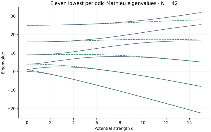
These are eigenvalues under one periodic boundary condition. They are not a complete Bloch band-structure calculation. Sorting at every \(q\) gives ordered eigenvalues; it does not transport a particular eigenvector continuously through crossings or near-degeneracies.
Change a physical parameter separately from resolution
openpfc run model.cpp input.json --source-root .. --launcher=noneinput.json selects n, q_max and the number of intervals in the sweep. results/mathieu.csv contains eleven modes at every sampled \(q\). Increase n while keeping the q sweep fixed before interpreting tiny separations. The checks recover the exact zero-potential multiplicities and compare a nonzero-q ground state with an independent Fourier-basis calculation. At coarse resolution, multiplication also aliases unresolved modes; the smoothness lesson explains why more digits in a solver output do not ensure more resolved physics.
The complete C++ model and starting input are available with this lesson. Keep the shared matrix.hpp one directory above the model.