Coupled fields / Ask each field for what you need

Two equations, two derivative requests, one sweep

Keep the equations visible. Change how the derivatives are evaluated.

Includes the model, inputs, required headers and a short run guide.

The runtime oscillator couples two fields without spatial derivatives. Now give each field a different derivative request. On the periodic cube \([0,2\pi)^3\), consider the numerical test model

\[ \begin{gathered} \begin{aligned} u_t &= v+a u_{xy},\\ v_t &= b\Delta u+c v_{xz}+d u_{yz}, \end{aligned}\\[4pt] (a,b,c,d)=\left(\frac3{10},\frac1{25},-\frac15,\frac2{15}\right). \end{gathered} \tag{1}\]

Here \(\Delta u=u_{xx}+u_{yy}+u_{zz}\). These coefficients give us an exact answer with every mixed term active. Write \(\phi=x+2y+3z\) and set \(u=A(t)\cos\phi\), \(v=B(t)\cos\phi\). Then \(u_{xy}=-2u\), \(u_{yz}=-6u\), \(v_{xz}=-3v\) and \(\Delta u=-14u\). The PDE reduces on this particular mode to

\[ \begin{gathered} \frac{d}{dt}\begin{pmatrix}A\\B\end{pmatrix} = M\begin{pmatrix}A\\B\end{pmatrix},\\[4pt] M=\begin{pmatrix}-0.6&1\\-1.36&0.6\end{pmatrix},\qquad M^2=-I. \end{gathered} \tag{2}\]

With \((A(0),B(0))=(1,0.6)\), this means \(A=\cos t\) and \(B=-\sin t+0.6\cos t\). Consequently the exact rates are \(u_t=-\sin t\cos\phi\) and \(v_t=(-\cos t-0.6\sin t)\cos\phi\). We evaluate a snapshot of those fields, rather than integrating them here. This separates spatial derivative errors from time-stepping errors. Oscillation of this one mode establishes no stability claim for arbitrary initial data or other Fourier modes of Equation 1.

Let the C++ types describe the requests

// Only these members are requested from either gradient backend.
struct UGrads {
  double xx{}, yy{}, zz{}, xy{}, yz{};
};
struct VGrads {
  double value{}, xz{};
};
struct Local {
  UGrads u;
  VGrads v;
};

u requests five derivatives; v requests its value and one derivative. Native evaluators recognize these member names. They supply physical spatial derivatives, including the grid-spacing factors. The model applies its coefficients once:

struct Model {
  Parameters parameters;
  OPENPFC_HD Increments rhs(double /*stage_time*/, const Local &g) const noexcept {
    const auto p = parameters;
    return {g.v.value + p.a * g.u.xy,
            p.b * (g.u.xx + g.u.yy + g.u.zz) + p.c * g.v.xz + p.d * g.u.yz};
  }
};

The returned aggregate opts into host tuple scatter:

struct Increments {
  double du{}, dv{};
  auto as_tuple() { return std::tie(du, dv); }
  auto as_tuple() const { return std::tie(du, dv); }
};

The order of the references in as_tuple() must match the output pointers. The types are ordinary model-owned C++ aggregates; neither a registry nor a string lookup is needed to describe the pointwise equations.

Prepare the right neighbours, then compose

pfc::comm::HaloExchangeOptions options;
options.connectivity = pfc::comm::HaloConnectivity::Full;
pfc::comm::HaloExchange<pfc::HostSpace, double> hu(u, decomposition, 0,
                                                   MPI_COMM_SELF, options);
options.exchange_base = 1;
pfc::comm::HaloExchange<pfc::HostSpace, double> hv(v, decomposition, 0,
                                                   MPI_COMM_SELF, options);
auto gu = pfc::gradient::FDGradient<coupled::UGrads>(
    u, 6, [&] { hu.exchange(); }, options.connectivity);
auto gv = pfc::gradient::FDGradient<coupled::VGrads>(
    v, 6, [&] { hv.exchange(); }, options.connectivity);

The sixth-order formulas need three halo layers. Mixed derivatives read off-axis neighbours, so the exchanges explicitly use Full connectivity. A face-only exchange would leave some required edge data stale. Separate exchange bases give the two fields distinct communication tags. This example uses one MPI process and periodic self-neighbours; it is a small way to exercise real halo preparation, rather than inventing a second boundary-fill implementation.

auto evaluator = pfc::field::create_composite<coupled::Local>(gu, gv);
std::vector<double> du(u.size()), dv(v.size());
pfc::sim::for_each_interior(
    coupled::Model{}, evaluator,
    std::make_tuple(du.data() + u.idx(0, 0, 0), dv.data() + v.idx(0, 0, 0)), time);

create_composite assembles Local{u,v} at each owned point. for_each_interior prepares the evaluator before the sweep, calls the model, and scatters its two increments. With padded FD fields, output pointers begin at the owned origin: evaluator indices are relative to that origin. The allocated output vectors still include the storage halo. Only owned rates are written to the CSV.

The same equation and output contract also accepts spectral gradients:

auto fft = pfc::fft::create(decomposition);
auto gu = pfc::field::create<coupled::UGrads>(u, fft);
auto gv = pfc::field::create<coupled::VGrads>(v, fft);
write_rates(gu, gv, u, v, time);

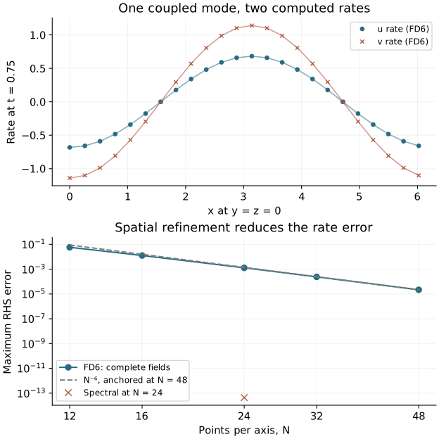
The transform plan is shared; each field evaluator prepares its own requested derivative arrays. This branch requires a HeFFTe-enabled CPU SDK. Its resolved Fourier mode has derivative error near floating-point roundoff.

Run, compare, and break a contract deliberately

Keep the shared equations header one directory above model.cpp. From this chapter’s directory run

openpfc run model.cpp input.json --source-root .. --launcher=none
openpfc run model.cpp spectral.json --source-root .. --launcher=none

The FD input chooses n, time, and method. The spectral input changes only the method. Both write all \(n^3\) owned rows to results/rates.csv: indices, coordinates, the two fields, computed rates and exact rates. The CLI prints each attempt’s output directory.

Double n from 24 to 48 at the same time. The leading FD rate error should fall by about \(2^6=64\). Change time to exercise a different combination of the two fields. The independent checker derives seven-point weights from exact polynomial moments and compares every rate with the resulting Fourier symbol, as well as checking the continuous answer.

For a staging experiment, read verify.hpp and verify.cpp. The preserved regression poisons input ghosts, changes the stage fields, checks an independent midpoint-mode recurrence, and checks that scatter leaves output ghosts untouched. A warmed-loop observer counts successful C++ new requests; it makes no claim about MPI pools or all system allocations. The optional HIP regression checks actual device evaluation and scatter with uploaded host-filled halos. This CPU tutorial does not execute a device stepper. The existing multi-field stepper limitations remain documented in #355; this lesson does not hide them inside a new integration wrapper.