Introduction
The Taylor–Green vortex is a closed test of a periodic incompressible solver. The initial velocity is one family of Fourier modes. Viscosity then generates smaller scales, dissipation rises to a peak near time 9, and the kinetic energy decays. Reynolds number 1600, formed with the unit velocity and the unit length of that trigonometric field, is the case used here. Viscosity is \(1/1600\).
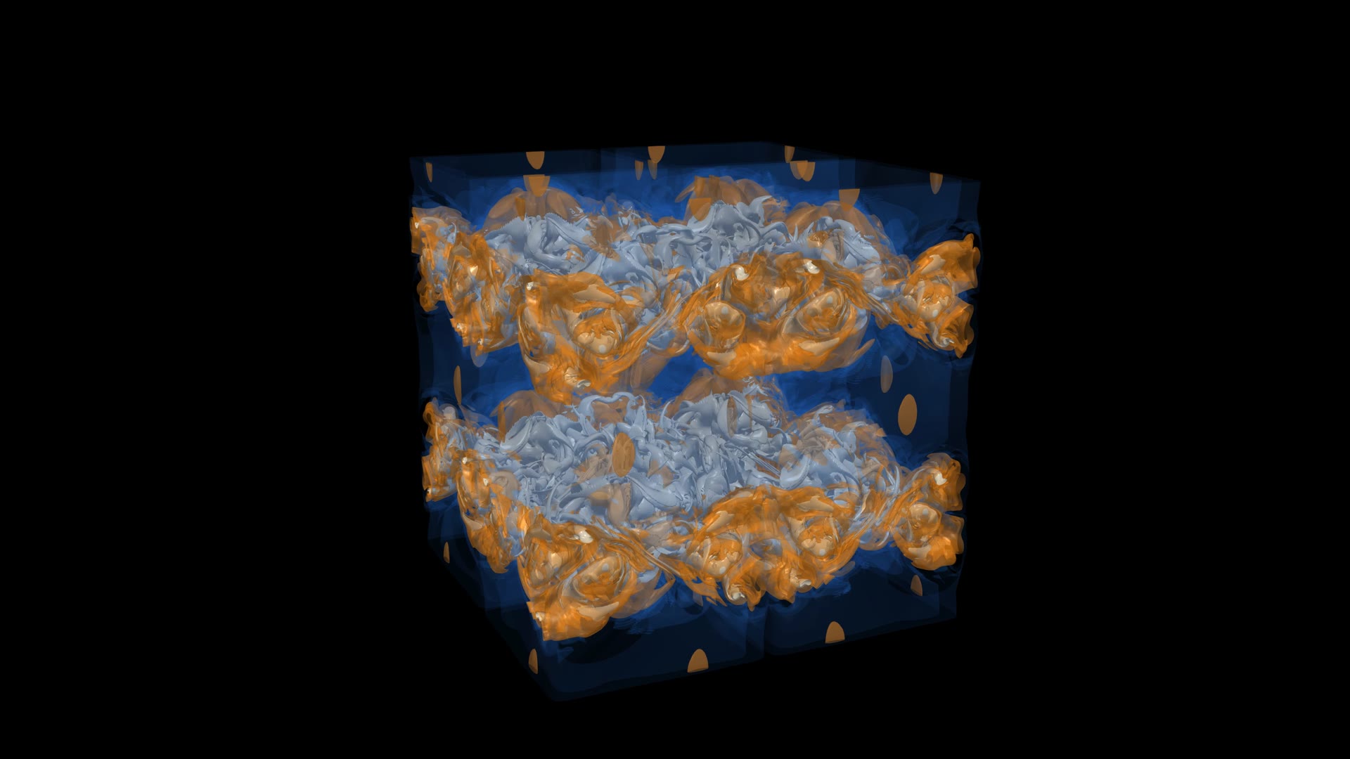
The calculation is the recorded \(512^3\) trajectory in OpenPFC. The film on this page is that run. The scalar comparison asks whether the same trajectory follows a public \(512^3\) pseudospectral table, and whether the grid is fine enough for those scalars. An inertial range, an ensemble mean, and a forced stationary state are outside that question.
The question
Does the periodic spectral step follow the public scalar table through the dissipation peak, and is \(512^3\) enough at this Reynolds number?
Through the peak, kinetic energy and viscous dissipation stay close to that table. A matched \(256^3\) run, decided against thresholds fixed before it started, moves the peak and the late decay by more than those thresholds allow. This page reports that recorded trajectory. A grid-converged benchmark is a further claim, and the grid comparison does not support it.
Governing equations
The domain is the cube \([0,2\pi]^3\). The velocity is periodic. With constant viscosity and no body force, the advance used by the application is
\[ \partial_t\hat{\mathbf u} = P(\mathbf u\times\boldsymbol\omega) - \nu|k|^2\hat{\mathbf u}. \tag{1}\]
\(P\) is the Fourier Leray projector, \(P = I - \mathbf{k}\mathbf{k}^{\mathsf T}/|k|^2\), on the odd wavevectors. A vanishing odd wavevector, including the mean, is left unchanged. The mean of the nonlinear tendency is set to zero, so an unforced mean velocity does not drift. Viscosity uses the same odd wavevector and is zero on those modes.
The rotational term is the projection of \(-(\mathbf u\cdot\nabla)\mathbf u\). On a divergence-free field the two agree, because \((\mathbf u\cdot\nabla)\mathbf u = \nabla(|\mathbf u|^2/2) - \mathbf u\times\boldsymbol\omega\) and \(P\) removes the gradient. The two-thirds mask is applied to the state before the product. A padded \(3/2\) product is not used.
Kinetic energy and enstrophy are
\[ E = \tfrac12\langle\mathbf u\cdot\mathbf u\rangle, \qquad \Omega = \langle\boldsymbol\omega\cdot\boldsymbol\omega\rangle, \qquad \varepsilon = \nu\Omega. \tag{2}\]
For this unforced scheme the projected rotational term does no work, so the balance on an exact sample is \(\mathrm dE/\mathrm dt = -\varepsilon\). Viscosity removes kinetic energy. The budget quoted below is the trapezoid of the recorded samples,
\[ E(T)-E(0)+\int\varepsilon\,\mathrm dt, \tag{3}\]
which tests that identity on the saved rows. It is separate from the agreement with the public table.
The initial field is
\[ u=\sin x\cos y\cos z,\qquad v=-\cos x\sin y\cos z,\qquad w=0. \tag{4}\]
Its cell averages are \(E=1/8\) and \(\Omega=3/4\), so the initial dissipation is \(4.6875\times10^{-4}\). The initial field is not isotropic, so a Taylor microscale is not used. The Kolmogorov scale is \(\eta=(\nu^3/\varepsilon)^{1/4}\). The retained cutoff \(k_{\max}\) is the largest integer strictly below \(N/3\): 170 at \(N=512\), and 85 at \(N=256\).
Numerical method
OpenPFC samples the velocity on a periodic structured grid and represents the derivatives in Fourier space. The viscous symbol is diagonal there. Integrating-factor RK4 removes that factor from the unknown and integrates the rotational term with classical RK4. HeFFTe distributes the transforms. The HIP build keeps the velocity and the Runge–Kutta stages on the device. A sample copies the coefficients back; the step itself stays on the device between samples.
Stored coefficients are unnormalised by \(N^3\). The modal divergence quoted below is \(|k\cdot\hat{\mathbf u}|/N^3\). The vorticity volumes used for the film are single-precision \(|\omega|\), one value per grid point, with \(x\) the fastest index. Those volumes cannot be turned back into a velocity spectrum.
The scheme controls the alias of a quadratic product by the two-thirds mask. It does not remove the error of a coarse grid or of a large step. Both of those are measured below.
Simulation setup
The filmed trajectory is one run. Length and time are the units of Equation 4, on the cube of side \(2\pi\).
| Quantity | Recorded run |
|---|---|
| Domain | Periodic cube, \([0,2\pi]^3\) |
| Grid | \(512^3\) |
| Viscosity | \(1/1600\), Reynolds number 1600 |
| Time step | \(1/960\) |
| Interval | \(t=0\) to \(t=20\), 19200 steps |
| Samples | Every \(1/60\), 1201 scalar rows |
| Volumes | Vorticity magnitude at the same interval, 1201 cubes |
| Initial energy | \(1/8\) |
| Initial enstrophy | \(3/4\) |
| Execution | HIP / HeFFTe, eight MI250X GCDs, one LUMI-G node |
| OpenPFC revision | 736ee45f |
A later build repeated the scalar samples and wrote shell spectra. Those scalars match the filmed run to a worst relative difference of 0 in kinetic energy, enstrophy, and dissipation. The comparison below uses that repeated table. The film still comes from the volumes of the original run.
Simulation results
The film is the recorded vorticity. Each frame is one stored volume. The volume at \(t=20\) is the unused endpoint, so the clip has 1200 frames. At 60 frames per second the playback lasts 20 seconds. The isosurfaces are vorticity magnitude 1, 5, and 12. The frame at \(t=9\) is the still at the top of the page.
Quantitative analysis
On the \(1/60\) samples the dissipation maximum is \(1.2858067\times10^{-2}\) at \(t=8.9833\). At that sample the kinetic energy is \(0.086618\) and the enstrophy is \(20.573\). At \(t=20\) the kinetic energy is \(0.021565\). The largest modal divergence on the samples is \(2.08\times10^{-17}\). The sample trapezoid (Equation 3) equals \(-7.00\times10^{-9}\). At the same peak, \(\eta=0.01174\) and \(k_{\max}\eta=1.996\) with \(k_{\max}=170\).
The public comparison is the workshop file spectral_Re1600_512.gdiag. Its header names a \(512^3\) spectral code. The columns are time, energy, \(-\mathrm dE/\mathrm dt\), and enstrophy. That enstrophy column equals \(0.375\) at \(t=0\), which is \(\langle|\omega|^2\rangle/2\). Viscous dissipation on both sides is \(\nu\langle|\omega|^2\rangle\), so the workshop enstrophy is doubled before the comparison. The file’s own \(-\mathrm dE/\mathrm dt\) column is a separate series. The workshop values are linearly interpolated onto the 1200 OpenPFC samples with \(t\le 19.99\). A relative difference uses the workshop value in the denominator.
| Window | Samples | Median \(\Delta E/E\) | Max \(\Delta E/E\) | Median \(\Delta\varepsilon/\varepsilon\) | Max \(\Delta\varepsilon/\varepsilon\) |
|---|---|---|---|---|---|
| \(t\in[0,5]\) | 301 | \(1.52\times10^{-8}\) | \(2.02\times10^{-7}\) | \(2.86\times10^{-6}\) | \(1.03\times10^{-5}\) |
| \(t\in[8,10]\) | 121 | \(1.89\times10^{-6}\) | \(1.29\times10^{-5}\) | \(4.35\times10^{-5}\) | \(5.01\times10^{-4}\) |
| \(t\in[15,19.99]\) | 300 | \(5.75\times10^{-4}\) | \(8.28\times10^{-4}\) | \(7.00\times10^{-4}\) | \(2.85\times10^{-3}\) |
| full overlap | 1200 | \(1.29\times10^{-5}\) | \(8.28\times10^{-4}\) | \(8.12\times10^{-5}\) | \(2.85\times10^{-3}\) |
Through the dissipation peak the integrated scalars follow the table. After \(t=15\) the gap is larger: up to \(8.3\times10^{-4}\) in energy and \(2.9\times10^{-3}\) in dissipation. The budget residual and the modal divergence measure this series. They do not measure agreement with the table. The value \(k_{\max}\eta\approx 2\) is a resolution diagnostic. It does not show that the tail has converged.
Numerical resolution
The same viscosity, the same step \(1/960\), and the same sample times were run at \(256^3\). Thresholds were fixed before that run. A peak dissipation that moves by more than \(3\times10^{-3}\) relative means \(512^3\) is not resolved for the peak. A maximum relative energy difference above \(1\times10^{-3}\) on \(t\ge 15\) means the late decay is not resolved at \(512^3\). A step of \(1/1920\) through \(t=10\), on the \(512^3\) grid, fails only if its dissipation peak moves by more than \(1\times10^{-4}\) relative.
| Comparison | Result | Threshold |
|---|---|---|
| Peak dissipation, \(256^3\) against \(512^3\) | \(4.32\times10^{-3}\) | \(3\times10^{-3}\) |
| Kinetic energy, \(t\ge 15\), maximum | \(2.15\times10^{-2}\) | \(1\times10^{-3}\) |
| Kinetic energy, \(t\ge 15\), median | \(1.35\times10^{-2}\) | |
| Dissipation peak, step \(1/1920\) | \(2.9\times10^{-12}\) | \(1\times10^{-4}\) |
The \(256^3\) dissipation peak is \(1.2913600\times10^{-2}\) at \(t=8.883\), against \(1.2858067\times10^{-2}\) at \(t=8.983\) on \(512^3\). Early kinetic energy, through \(t=5\), differs by a median relative \(1.9\times10^{-12}\). The gap appears as the smaller scales grow. The halved step keeps the same peak time, and the peak value moves by \(2.9\times10^{-12}\) relative. The step is adequate for the peak. The grid misses both spatial thresholds.
\(k_{\max}\) is 85 on the coarser grid and 170 on \(512^3\). Shells above 85 have no \(256^3\) neighbour. Shell spectra were written for both grids and are not plotted here. The scalar thresholds already answer the question this page asks: \(512^3\) is not resolved for the dissipation peak or for the late decay.
Performance
The filmed \(512^3\) run used eight graphics compute dies on one LUMI-G node. It ran for 11 hours 16 minutes, about 2.11 seconds a step. That interval includes writing a vorticity volume at every sample.
A separate window of 40 profiled steps at \(1024^3\), with volume output left off, measured the step on 8, 16, 32, and 64 dies. The profile synchronises the device, so the times are upper bounds. The fast Fourier transform is most of each step. Device state for that grid is 272 GiB. From 8 to 16 dies the step drops by a factor of about 5. Each further doubling runs at about 80 percent efficiency.
| Dies | Step (s) | GPU-hours to \(t=20\) | Wall time |
|---|---|---|---|
| 8 | 11.34 | 484 | 60 h |
| 16 | 2.24 | 191 | 12 h |
| 32 | 1.39 | 237 | 7.4 h |
| 64 | 0.874 | 298 | 4.7 h |
Sixteen dies is the cheapest width that fits in that maximum. An integration to \(t=20\) there is about 191 GPU-hours, with diagnostics and shell spectra and without a volume sequence. A later attempt at that width was given 20 hours. It wrote the initial sample and no later sample. There is no \(1024^3\) trajectory on this page.
What the application does and does not do
What it does
- Periodic incompressible Navier–Stokes on a cube.
- The Taylor–Green initial condition at Reynolds number 1600.
- A Fourier Leray projector and a state-level two-thirds mask.
- Integrating-factor RK4, with HIP and HeFFTe on the filmed run.
- Kinetic energy, enstrophy, dissipation, and modal divergence.
- Shell spectra on the repeated scalar run.
- Vorticity-magnitude volumes, which are the frames of the film.
What it does not do
- Establish a grid-converged benchmark. The \(256^3\) comparison misses the thresholds for the peak and for the late decay.
- Treat walls, inflow, or a pipe. The filmed run is periodic and unforced.
- Report an inertial range, an ensemble mean, or a forced stationary state.
- Show a finished \(1024^3\) trajectory. That attempt stopped after the initial sample.
- Reconstruct the velocity from the film. Each frame stores \(|\omega|\) only.
The public table is a numerical comparison. Agreement through the peak, and the miss at late time, are both properties of this one trajectory.