OpenPFC / Operators and their solutions
A contour turns an integral into a sum
Use complex arithmetic and a shifted trapezoidal rule to approximate reciprocal gamma, while keeping poles and branch choices explicit.
Download runnable lesson (.zip)
Includes the model, inputs, required headers and a short run guide.
Program 31 of Trefethen (2000) draws the complex gamma function using a short contour sum. The underlying identity is Hankel’s representation of the reciprocal gamma function, documented in National Institute of Standards and Technology (n.d.):
\[\frac1{\Gamma(z)}=\frac1{2\pi i}\int_{-\infty}^{(0+)} e^t t^{-z}\,dt.\]
The contour travels from the negative real axis, circles zero in the positive direction and returns along the other side. A branch choice is part of this formula, not an implementation afterthought.
Parameterize once, then sample
Use the book’s circle \(t(\theta)=-11+16e^{i\theta}\). Since \(dt=i(t+11)\,d\theta\), a midpoint-shifted trapezoidal sum gives
\[ \begin{gathered} G_N(z)=\frac1N\sum_{j=0}^{N-1}e^{t_j}t_j^{-z}(t_j+11), \\ \theta_j=-\pi+\frac{2\pi}{N}(j+\tfrac12). \end{gathered} \]
Complex reciprocal_gamma(Complex z, int samples) {
  constexpr double center = -11, radius = 16;
  Complex sum = 0;
  for (int j = 0; j < samples; ++j) {
    const double theta =
        -std::numbers::pi + 2 * std::numbers::pi * (j + .5) / samples;
    const Complex t = center + radius * std::exp(Complex(0, theta));
    sum += std::exp(t - z * std::log(t)) * (t - center);
  }
  return sum / static_cast<double>(samples);
}
std::complex expresses the formula directly. The principal complex logarithm and half-grid shift avoid evaluating exactly on the negative-real branch cut. The finite circular path also truncates the two negative-axis tails. Increasing N controls sampling error, not that independent contour truncation. The sum is a mathematical reference using the standard library; it does not claim a public OpenPFC special-function API.
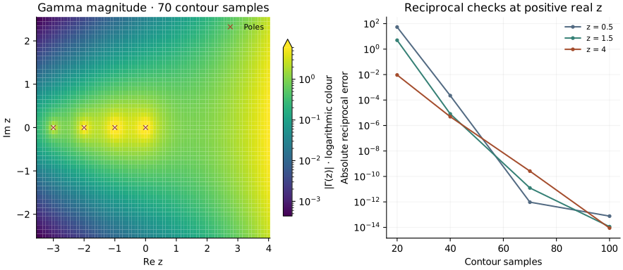
A pole is not a very large finite answer
openpfc run model.cpp input.json --launcher=noneThe default uses 70 samples and the original complex rectangle. The CSV records the raw reciprocal estimate and marks exact nonpositive-integer poles on the real axis. Gamma magnitude there is NaN by design, rather than a finite height obtained by dividing roundoff noise into one. results/convergence.csv also includes 20,40,70,100-point sums at positive real arguments with factorial and half-integer checks.
Conjugate symmetry is checked across the rectangle. The recurrence check uses \(0.5\le\Re z\le3\), so that \(z+1\) stays in the output; its tolerance reflects the 70-point quadrature. Real-axis checks require substantial improvement from 40 to 70 samples, and agreement within \(10^{-11}\) at 100 samples. The default experiment is not a uniform high-precision special function implementation over the entire rectangle. Cancellation, branch-cut tails and proximity to poles all affect the answer. This is an opportunity to ask what each numerical limit actually controls.
The complete C++ model and starting input are available with this lesson.