Let the field determine its own forcing

Polynomial methods / Learn by experiment

Let the field determine its own forcing

Solve a nonlinear boundary-value problem using OpenPFC Newton–GMRES, then check it with a scalar root and an analytic solution.

Download runnable lesson (.zip)

Includes the model, inputs, required headers and a short run guide.

Replace the prescribed forcing by the unknown field itself:

\[ \begin{gathered} u''=e^u, \\ u(-1)=u(1)=0. \end{gathered} \tag{1}\]

Program 14 of Trefethen (2000) solves this problem by fixed-point iteration. We keep its equation, Chebyshev grid and degree 16, and use OpenPFC’s Newton–GMRES solver instead. This is an explicit change of nonlinear algorithm, with an independent solution available to judge the result.

State the residual and its derivative

After removing the known endpoints, write \(F(u)=D^2u-e^u\). Newton’s correction satisfies

\[ \begin{gathered} J(u)\,\delta=-F(u), \\ J(u)v=D^2v-e^u v. \end{gathered} \tag{2}\]

The final product is componentwise. The model provides residual, linearization, Jacobian action and a diagonal inverse preconditioner.

struct BoundaryProblem {
  polynomial::Matrix d2;
  polynomial::Vector exponential;
  void residual(const auto &u, auto &r) {
    r = polynomial::apply(d2, u);
    for (std::size_t i = 0; i < u.size(); ++i) r[i] -= std::exp(u[i]);
  }
  void linearize(const auto &u) {
    exponential.resize(u.size());
    for (std::size_t i = 0; i < u.size(); ++i) exponential[i] = std::exp(u[i]);
  }
  void jacobian(const auto &v, auto &jv) {
    jv = polynomial::apply(d2, v);
    for (std::size_t i = 0; i < v.size(); ++i) jv[i] -= exponential[i] * v[i];
  }
  void precondition(const auto &r, auto &z, int) {
    z.resize(r.size());
    for (std::size_t i = 0; i < r.size(); ++i)
      z[i] = r[i] / (d2[i][i] - exponential[i]);
  }
  // This model caches only the Jacobian at the accepted iterate.
  void begin_trial(const auto &) {}
  void accept_trial(const auto &) {}
  void reject_trial() {}
};

The trial hooks are empty because evaluating this model has no persistent trial state. A material model that caches history would need to implement those hooks so rejected trials cannot alter its accepted state.

Solve the actual equations

pfc::solvers::VectorOperations<> ops;
pfc::solvers::NewtonControls controls;
controls.relative_tolerance = 1e-11;
controls.absolute_tolerance = 1e-11;
controls.linear.restart = n - 1;
polynomial::Vector interior(n - 1);
const auto result = pfc::solvers::newton(ops, model, interior, controls);
if (!result.converged()) throw std::runtime_error("Newton did not converge");

OpenPFC chooses an inexact linear tolerance and uses a line search to admit a correction. A small change in the iterate is not our convergence test: the nonlinear residual must satisfy the stated tolerances. The initial interior field is zero, already consistent with the boundary data.

Derive a reference without a second collocation solve

Try \(u(x)=2\log[\cos(a)/\cos(ax)]\). Then \(u''=2a^2\sec^2(ax)\) and \(e^u=\cos^2(a)\sec^2(ax)\), so the positive parameter satisfies

\[ \begin{gathered} \cos a=\sqrt2\,a, \\ 0<a<1. \end{gathered} \tag{3}\]

OpenPFC’s safeguarded scalar root finder supplies \(a\). Its function value and derivative are only a few characters:

const auto parameter = pfc::solvers::scalar_root(
    [](double a) {
      return pfc::solvers::ScalarValue{std::cos(a) - std::sqrt(2.0) * a,
                                       -std::sin(a) - std::sqrt(2.0)};
    },
    0.0, 1.0, 0.5);
if (!parameter.converged()) throw std::runtime_error("Reference root failed");
auto exact = [&](double point) {
  return 2 * std::log(std::cos(parameter.x) / std::cos(parameter.x * point));
};

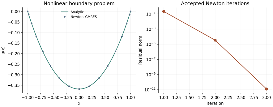
The independent regression uses bisection for this scalar equation and compares every recorded point, so agreement is not inferred from the Newton residual alone.

Figure 1: The nonlinear solution and its analytic reference, followed by the residual of each accepted Newton iteration.

Look at convergence as well as the final curve

openpfc run model.cpp input.json --source-root .. --launcher=none

The attempt writes results/nonlinear.csv and results/newton.csv. The second file records accepted residuals, step lengths and inner linear iterations. Increase n to 24 and distinguish improved spatial accuracy from a tighter nonlinear solve. An indefinitely tighter tolerance can encounter cancellation in \(D^2u\), whose entries grow strongly near the endpoints. A reported solve failure should remain visible, not be hidden by silently relaxing the tolerance.

The complete C++ model and starting input are available with this lesson. It also uses the shared collocation.hpp; keep its relative location when saving the files.

References

Trefethen, Lloyd N. 2000. Spectral Methods in MATLAB. Society for Industrial; Applied Mathematics. https://doi.org/10.1137/1.9780898719598.