Materials / Recover a macroscopic law from a small cell
Let layers choose two different averages
Six imposed strains. Six averaged stresses. A layered solution to check them.
Download runnable lesson (.zip)
Includes the model, inputs, required headers and a short run guide.
An elastic cell can have a simple local law and a direction-dependent macroscopic response. On the periodic cube \([0,2\pi)^3\), let the two Lamé coefficients vary only along \(x\):
\[ \lambda(x)=\mu(x)=\frac{1}{1+a\cos x}. \]
Choose \(0\le a\le1/2\). All values are nondimensional. Each point is locally isotropic, with \(\boldsymbol\sigma=\lambda\operatorname{tr}(\boldsymbol\varepsilon)I +2\mu\boldsymbol\varepsilon\). The cell is graded continuously; the stiffness weight below is not a binary phase indicator.
Describe the material with an ordinary field
SpectralCPUStack supplies a domain, owned field and distributed FFT. The homogenizer interpolates linearly between two positive stiffnesses, so we express the prescribed \(\mu(x)\) through their shared scalar weight:
const double soft = 1 / (1 + amplitude), hard = 1 / (1 - amplitude);
weight.apply([&](double x, double, double) {
  const double mu = 1 / (1 + amplitude * std::cos(x));
  return amplitude == 0 ? 0.0 : (mu - soft) / (hard - soft);
});
pfc::solvers::MicroelasticityParams parameters;
parameters.stiffness_at_zero = pfc::solvers::Stiffness::from_lame(soft, soft);
parameters.stiffness_at_one = pfc::solvers::Stiffness::from_lame(hard, hard);
parameters.relative_tolerance = 1e-11;
parameters.max_iterations = 200;
parameters.comm = comm;
from_lame receives \(\lambda\) and \(\mu\) directly. At \(a=0\) both endpoints coincide; assigning zero weight avoids a zero denominator and recovers a homogeneous material.
Ask the same cell six independent questions
For each imposed mean strain \(\bar{\boldsymbol\varepsilon}\), solve
\[ \begin{aligned} \nabla\cdot\boldsymbol\sigma&=0,\\ \boldsymbol\varepsilon &=\bar{\boldsymbol\varepsilon} +\operatorname{sym}\nabla\mathbf u^\#,\\ \langle\operatorname{sym}\nabla\mathbf u^\#\rangle&=0, \end{aligned} \]
where the displacement fluctuation \(\mathbf u^\#\) is periodic. There is no eigenstrain in these unit-load solves. FFT-based composite solvers use a homogeneous reference medium’s Green operator to update the heterogeneous cell (Moulinec and Suquet 1998). The example composes OpenPFC’s installed implementation:
pfc::solvers::PeriodicHomogenizer homogenizer(domain, stack.fft(), parameters);
const auto effective = homogenizer.compute(weight);
if (!effective.all_converged())
  throw std::runtime_error("A unit-load elasticity solve did not converge");
The solver’s default accelerated fixed point reports relative polarization change. The example sets its tolerance to \(10^{-11}\) and rejects an unconverged load. That stopping measure is not an independent field-error bound; the layered solution below supplies a separate check.
Be explicit about shear
The effective matrix acts on the engineering strain vector
\[ (\varepsilon_{11},\varepsilon_{22},\varepsilon_{33}, \gamma_{23},\gamma_{13},\gamma_{12})^T, \]
with \(\gamma_{ij}=2\varepsilon_{ij}\). The library’s Sym3 fields store tensor shear, so a unit engineering-shear load imposes mean tensor shear \(1/2\). An isotropic engineering shear diagonal is \(\mu\), not \(2\mu\).
To derive the response for the last load, impose \(\bar\gamma_{12}=1\). Layered equilibrium makes \(\sigma_{12}=S\) constant, while \(\varepsilon_{12}=S/(2\mu(x))\). Averaging the engineering strain gives
\[ 1=S\langle1/\mu\rangle, \qquad H=\langle1/\mu\rangle^{-1}=1. \]
Thus the exact local fields are
\[ \sigma_{12}=1,\qquad \varepsilon_{12}(x)=\tfrac12(1+a\cos x). \]
Softer layers take more strain under the same stress. Shear parallel to the layers, \(\gamma_{23}\), instead has constant strain and averaged stress proportional to the arithmetic mean of \(\mu\).
const auto &strain =
    homogenizer.strain(pfc::solvers::SYM_XY)[pfc::solvers::SYM_XY];
const auto &stress = homogenizer.solver().stress()[pfc::solvers::SYM_XY];
std::ofstream field("results/field_rank_" + std::to_string(comm.rank()) +
                    ".csv");
if (!field) throw std::runtime_error("Cannot open local shear field");
field << std::setprecision(17) << "x,y,z,weight,epsilon_xy,sigma_xy\n";
strain.for_each_owned([&](int i, int j, int k) {
  const auto x = strain.coords(i, j, k);
  field << x[0] << ',' << x[1] << ',' << x[2] << ',' << weight(i, j, k) << ','
        << strain(i, j, k) << ',' << stress(i, j, k) << '\n';
});
strain(load) retains each solved total strain. After the six loads, solver().stress() belongs to the last load, engineering \(12\) shear; the code reads the matching tensor components from both.
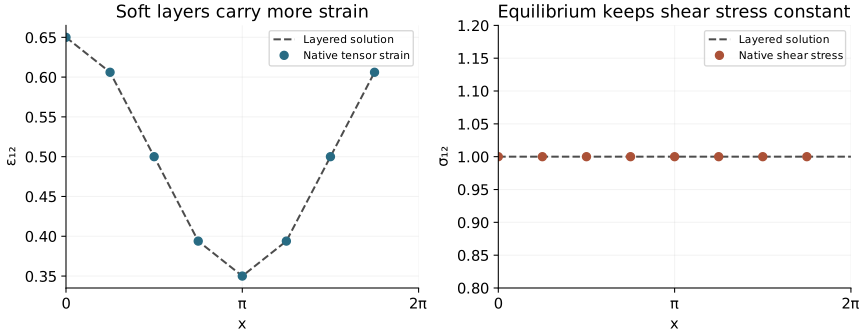
The plot uses actual C++ fields on one owned grid line. Output checks visit every node from every rank, not only this line.
Check the entire effective tensor
Define the grid arithmetic mean
\[ A_N=\frac1N\sum_{i=0}^{N-1} \frac{1}{1+a\cos(2\pi i/N)}. \]
Normal equilibrium also makes \(\sigma_{11}\) constant. Since \(\sigma_{11}=\mu(3\varepsilon_{11}+\bar\varepsilon_{22} +\bar\varepsilon_{33})\), solving for \(\varepsilon_{11}\) and averaging gives \(\sigma_{11}=3\bar\varepsilon_{11}+\bar\varepsilon_{22} +\bar\varepsilon_{33}\). Define \(b=(1+8A_N)/3\) and \(c=(1+2A_N)/3\). The normal block is
\[ C_{\mathrm{normal}}= \begin{pmatrix} 3&1&1\\ 1&b&c\\ 1&c&b \end{pmatrix}. \]
The engineering shear diagonals, in \(23,13,12\) order, are \((A_N,1,1)\). All other entries are zero. At \(a=0\), \(A_N=1\) and the homogeneous isotropic tensor is recovered.
The continuum arithmetic mean is \(1/\sqrt{1-a^2}\). A finite grid uses the discrete \(A_N\), which approaches that integral as resolution increases. This distinction matters even when the iterative solve is accurate. The compatible layered strains above are represented by the constant and first cosine mode; their nodal constitutive stresses give this discrete tensor without requiring a second FFT solver as an oracle.
The checker compares all 36 effective entries and the unsymmetrized mean stress columns, checks the six mean strains and verifies complete nodal ownership and local shear fields. A converged iteration alone would not establish these properties.
Run the cell and change its contrast
From the repository root, with a compatible installed spectral CPU SDK:
openpfc run examples/materials/layered-homogenization/model.cpp examples/materials/layered-homogenization/input.jsonThe CLI prints its saved attempt directory. Under its results/, inspect stiffness.csv, run.json and field_rank_*.csv. To run the same model on two ranks, add --ranks 2 --launcher=mpirun to the source-run command; invoke the CLI once outside the launcher.
The complete model and input need no private helper headers. The CMake target is layered_homogenization.
Start with amplitude zero and predict all tensor entries. Then restore 0.3, compare the two shear averages and repeat at n equal to 16. Separate iterative error, grid averaging and material contrast when interpreting those differences. This small linear elastic cell does not establish performance or accuracy for high-contrast or nonlinear materials.