An FFT reads the memory you give it

Fourier methods / Match the plan and its buffers

An FFT reads the memory you give it

Change the backend. Keep the field, ownership and normalization contracts.

Download runnable lesson (.zip)

Includes the model, inputs, required headers and a short run guide.

The first FFT lesson checks what a transform means. Here the question is where its arrays live. A host std::vector and a device allocation can have the same number of doubles, but an FFT must receive the kind of memory its backend expects.

Use the periodic box \([0,L_x)\times[0,L_y)\times[0,L_z)\) and sample \(u(x,y,z)\):

\[ \begin{aligned} u&=1+0.3\cos(2\pi x/L_x)\\ &\quad+0.2\sin(4\pi y/L_y)\cos(2\pi z/L_z). \end{aligned} \]

double signal(double x, double y, double z, const Parameters &p) {
  const double tau = 2 * std::numbers::pi;
  return 1 + 0.3 * std::cos(tau * x / p.length[0]) +
         0.2 * std::sin(2 * tau * y / p.length[1]) * std::cos(tau * z / p.length[2]);
}

Coordinates come from the owned global grid, rather than a rank-local flat index. Changing the MPI decomposition therefore changes ownership, not the function being transformed. No endpoint is duplicated: spacing is \(L_d/N_d\) along each axis.

Start with a host plan and host arrays

auto fft = pfc::fft::create(decomposition, comm.rank());
auto real = initial;
std::vector<std::complex<double>> modes(fft.size_outbox());
for (int pass = 0; pass < p.cycles; ++pass) {
  fft.forward(real, modes);
  fft.backward(modes, real);
}
return {std::move(real), std::move(modes), fft.get_outbox_bounds()};

Both vector lengths come from the plan. The real inbox and complex outbox can differ in size and decomposition. The forward transform is unscaled; the inverse includes division by the total global number of real cells, \(M=N_xN_yN_z\). One forward/backward pair therefore returns \(u\), and repeated pairs should keep returning \(u\) up to roundoff. A missing inverse scale would amplify the field by \(M\) on every pass.

All MPI ranks must construct the plan and execute every transform in the same sequence. A distributed FFT can exchange data even while its result is needed only on rank zero. The original timing demonstrator guarded plan construction and execution with rank == 0; this lesson removes that collective-participation error. Rank zero only writes the global summary.

Give a device plan device buffers

template <class Tag, class FFT, class Synchronize>
Result round_trip_device(FFT &fft, const std::vector<double> &initial, int cycles,
                         Synchronize synchronize) {
  pfc::core::DataBuffer<Tag, double> real(fft.size_inbox());
  pfc::core::DataBuffer<Tag, std::complex<double>> modes(fft.size_outbox());
  real.copy_from_host(initial);
  for (int pass = 0; pass < cycles; ++pass) {
    fft.forward(real, modes);
    fft.backward(modes, real);
  }
  synchronize();
  return {real.to_host(), modes.to_host(), fft.get_outbox_bounds()};
}

DataBuffer<Tag,T> owns backend-specific storage. For the device tags in this function, copy_from_host uploads the local real input, and to_host downloads the final values and coefficients. The transforms remain on the device between those transfers. Host indexing such as real[i] is not a substitute for a device kernel.

The CUDA branch chooses its native factory and checks execution completion:

auto fft = pfc::fft::create_cuda(decomposition, comm.rank(), comm);
return round_trip_device<pfc::backend::CUDATag>(fft, initial, p.cycles, [] {
  if (cudaDeviceSynchronize() != cudaSuccess)
    throw std::runtime_error("CUDA FFT execution failed");
});

The HIP branch has the same structure, using HIPTag, create_hip and hipDeviceSynchronize. The code binds each rank to a visible local device before constructing its GPU plan. On a cluster, visibility and allocation come from the scheduler; device zero means the first device visible to that rank. Backend selection never silently falls back to CPU.

The synchronization check completes queued work before observing it on the host. These are correctness boundaries, not a timing protocol. This example makes no speedup or hardware recommendation from a small run. The stable executable name fft_backend_benchmark is retained for existing build users, but its current purpose is the numerical backend experiment.

Know the answer before comparing backends

Write the normalized Fourier coefficient as \(c_{ijk}=\widehat u_{ijk}/M\). Euler’s identity gives all the nonzero coefficients:

Mode	Normalized coefficient
\((0,0,0)\)	\(1\)
\((\pm1,0,0)\)	\(0.15\)
\((0,2,\pm1)\)	\(-0.05i\)
\((0,-2,\pm1)\)	\(+0.05i\)

The real-to-complex plan stores only \(0\leq i\leq\lfloor N_x/2\rfloor\). Negative indices on the other axes are represented by their residues, such as \(N_y-2\). The missing negative-\(i\) partners are reconstructed by complex conjugacy. Consequently

\[ \begin{aligned} \langle u\rangle&=1,\\ \langle u^2\rangle&=1+2(0.15)^2\\ &\quad+4(0.05)^2=1.055. \end{aligned} \]

Parseval’s identity gives the same mean square from the compressed spectrum, weighting its interior-\(i\) coefficients twice. The \(i=0\) plane and an even grid’s \(i=N_x/2\) plane each have weight one. Testing all coefficients, including the expected zeros, exposes normalization or layout errors that a plausible-looking field alone might hide.

Figure 1: Native prescribed and CUDA-recovered nodal cross-sections, followed by the measured CPU and CUDA return errors on one grid line.

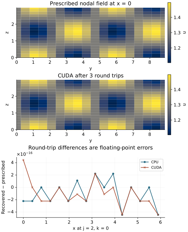
These plots read the C++ CSV files. The first two panels use the same color scale and the actual \(x=0\) nodes. The errors in the last panel measure returning the prescribed input, rather than a PDE’s spatial truncation error. The independent checks also inspect the complete fields and spectra outside these displayed cross-sections.

Run the same experiment in different memory

With a compatible installed spectral CPU SDK:

openpfc run model.cpp input.json --launcher=none
openpfc run model.cpp input.json --ranks=2 --launcher=mpirun

The C++ model and CPU input use a small rectangular grid and three round trips. The printed attempt contains results/field_rank_<rank>.csv, modes_rank_<rank>.csv and summary.json. Both distributed layouts carry global indices. The summary reports the actual field error, mean and mean square.

The source-model CLI currently qualifies CPU execution. For the GPU route, build from the checkout using the supported script and run its executable inside a suitable allocation:

./scripts/build.sh --machine=tohtori --with-cuda --build-dir=builds/cuda
builds/cuda/examples/fft_backend_benchmark examples/fourier/backend-buffers/cuda.json

Run GPU commands inside a suitable allocation. On LUMI use ./scripts/build.sh --machine=lumi --with-rocm --wait, then the executable from the configured flash build with hip.json on an allocated GPU node. The CUDA input and HIP input change only backend; they require their matching spectral backend in the build. See the installation guide for the compiler, MPI, HeFFTe and accelerator stack.

Change shape to an odd grid or increase cycles. The physical field and known coefficients stay fixed; the accumulated roundoff need not match bit for bit between FFT libraries or decompositions. Compare the complete outputs and the analytic coefficients, rather than accepting parity between two potentially incorrect implementations. The native checker uses those independent coefficients and verifies every real and spectral owner exactly once.

For a model change, replace the amplitudes \(0.3\) and \(0.2\) by \(a\) and \(b\). Predict \(\langle u^2\rangle=1+a^2/2+b^2/4\) before running. The checker is for the prescribed experiment: when you change the signal, rederive its coefficient table and moment checks as well.